In this article, we will analyse the fire resistance of a reinforced concrete slab. We will use the Eurocode as reference in this example.
Fire resistance is the ability of a structural system, a part of it, or an individual element to fulfill its required functions (such as load-bearing capacity and/or compartmentation/enclosing functions) for a specified fire exposure and for a specified period of time.
When exposed to the standard fire exposure (i.e., ISO 834), the term standard fire resistance is used.
The standard fire resistance of a reinforced concrete slab is defined by the R, E, I classification.
R is the load-bearing capacity, which is the ability to withstand mechanical loads without collapsing.
E is for integrity, which is the ability to prevent the passage of flames and hot gases through cracks or openings.
I is the insulation, which is the ability to limit temperature rise on the unexposed side (i.e., 140 K average or 180 K max limits).
The minimum slab thickness and reinforcement axis distance for each fire resistance class are shown in the following table assuming a simply-supported slab.
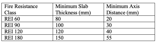
In this example, we will model a reinforced concrete slab with a standard fire resistance of REI 90, meaning the slab can resist a fire for a period of at least 90 minutes under the standard fire curve exposure.
Problem Definition and Assumptions
The slab arrangement and boundary conditions are illustrated in the diagram below.
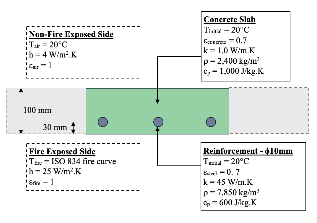
Based on the physical arrangement and exposure conditions, the heat transfer process can be modelled as transient and one-dimensional under the following assumptions:
Radiation & Convection: Radiative and convective heat transfer uniformly across the fire and non-fire exposed surfaces of the concrete slab.
Exposure Condition: ISO 834 fire curve, which is expressed as Tfire = 345 log10(8t + 1) + 20, where t is in minute.
One-Dimensional Flow: Temperature gradients and heat flux in the horizontal (x-axis) and depth (z-axis) directions are negligible.
Transient Problem: The system represents short-term heat transfer per unit area under fire exposure.
It is noted that the thermal properties of the concrete and reinforcement in reality will vary with temperature. However, in this example we will assume that the thermal properties are constant irrespective of the temperature.
The .txt input file for the HeatCond2D model is available for download here.
If you have any queries or feedback regarding this article, please contact us.
Step-by-Step Heat Transfer Analysis
We will start by creating the reinforced concrete slab section.
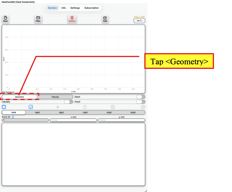
Open the HeatCond2D app and tap on the Section Page. Ensure that <Geometry> is selected.
Section Page
Tap <Geometry>
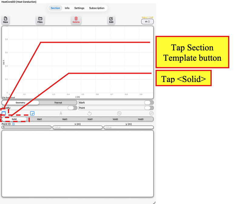
Tap <Solid> to ensure that the Solid Element is selected. The Solid Element will represent the concrete slab
Next, tap the Section Template button to access the Section Template Page.
Section Page
Tap <Solid>
Tap Section Template button
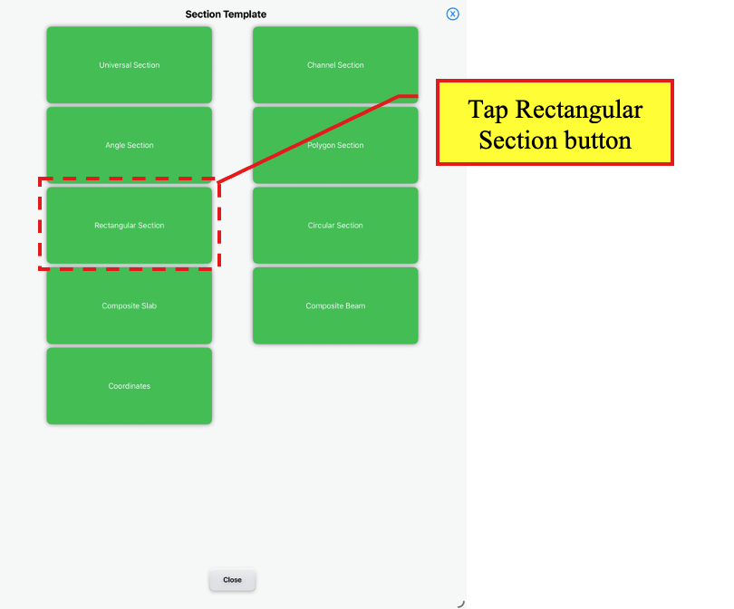
On the Section Template Page, tap the Rectangular Section button to access the template for a rectangular section.
Section Template Page
Tap Rectangular Section button
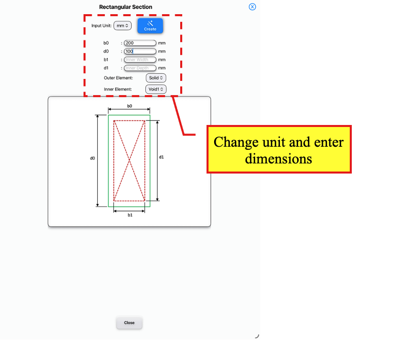
Under Input Unit, select mm to change the unit.
Then, enter the following dimensions:
b0 = 200 in mm
d0 = 100 in mm
leave b1 and d1 empty.
Ensure that the Outer Element and Inner Element are set to Solid and Void1 respectively.
Rectangular Section Template
Change unit and enter dimensions
Tap the Scribble button to create the rectangular section.
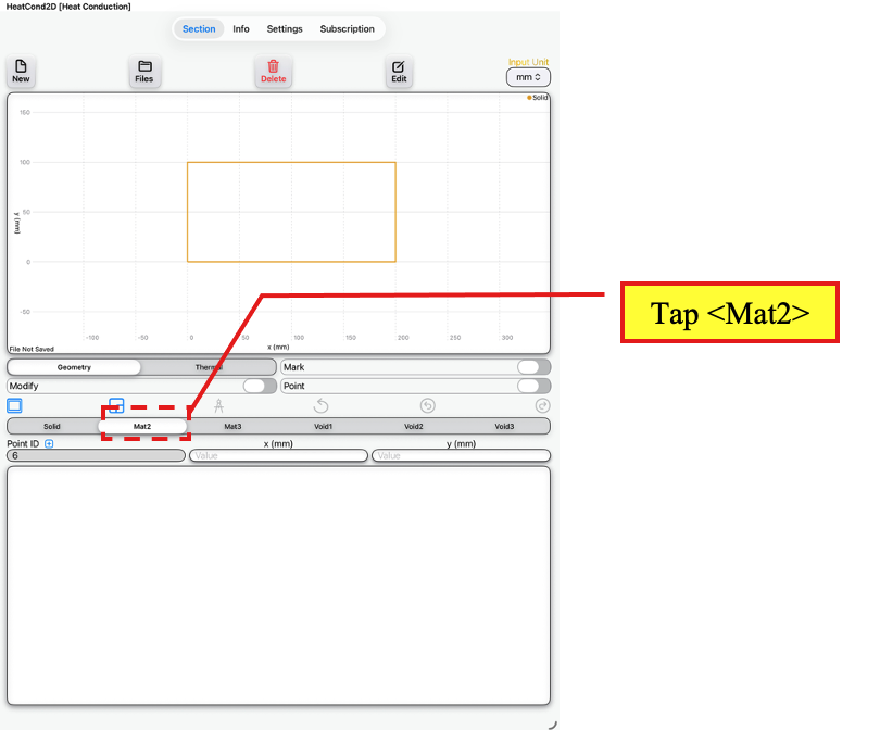
Back on the Section Page, tap <Mat2> which will represent the reinforcement bar.
Section Page
Tap <Mat2>
Tap on the Shape Template button to access the Shape Template Page.
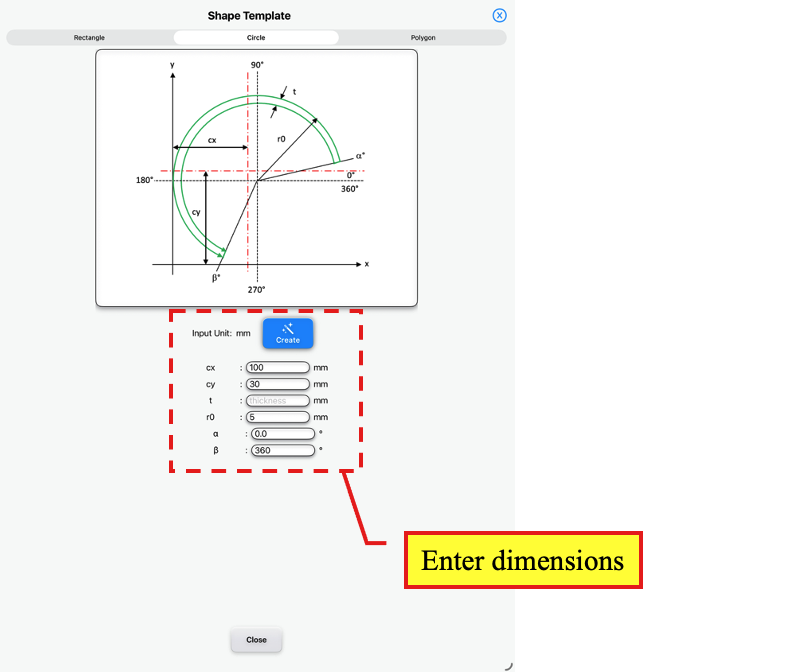
Tap <Circle> and enter the following dimensions:
cx = 100 in mm
cy = 30 in mm
r0 = 5 in mm
leave t, α and β empty.
Shape Template
Tap <Circle>
Enter dimensions
Tap <Create> to create the shape and return to the Section Page.
Next, we will create the heat transfer model. On the Section Page, toggle on the Thermal toggle button to access the Thermal Page.
We will then generate the meshes for the model. Tap on the Mesh Properties button to access the Mesh Properties Page.
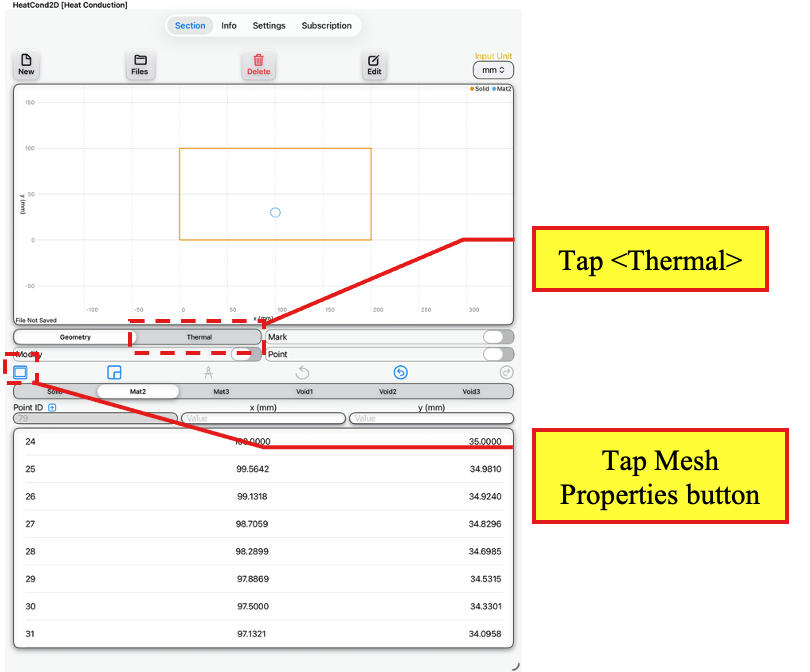
Section Page →Thermal Page
Tap <Thermal>
Tap Mesh Properties button
We will use symmetry modelling for this example.
On the Mesh Properties Page, tap on the Symmetry button to access the Symmetry Modelling Page.
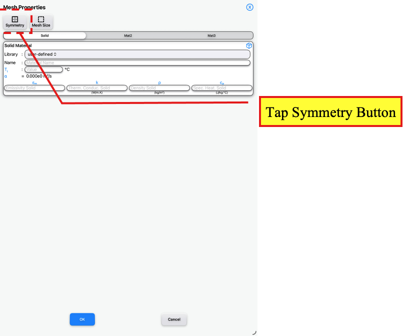
Mesh Properties Page
Tap Symmetry button
On the Symmetry Modelling Page, tap the ‘NorthWest Corner’ and ‘SouthWest Corner’ buttons.
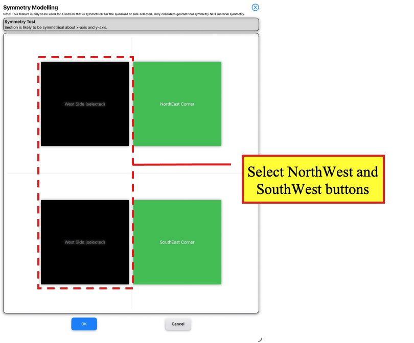
Symmetry Modelling
Tap NorthWest and SouthWest buttons
Tap the OK button to return to the Mesh Properties Page.
On the Mesh Properties Page, tap the Mesh Size button to access the Mesh Size Page.
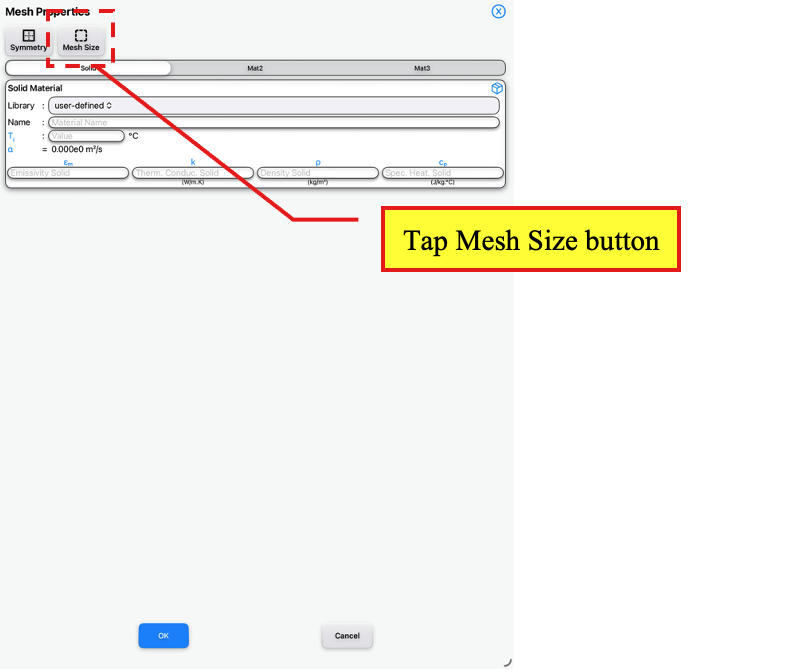
Mesh Properties Page
Tap Mesh Size button
Enter Δx of 5 in mm and Δy of 5 in mm. Leave Mesh Symmetry as “About y- and x- axes and Selected Mesh Size as “Modified Mesh Size”.
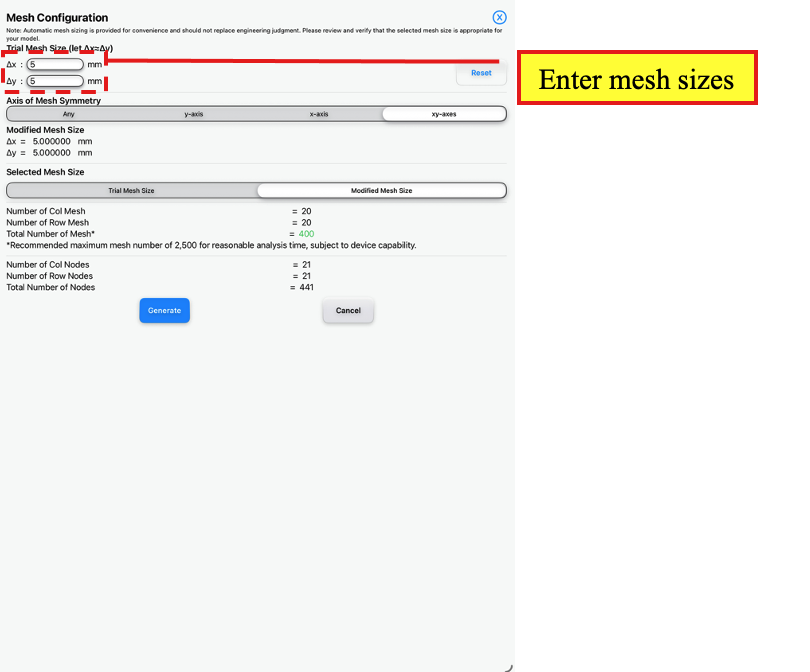
Mesh Size Page
Enter mesh sizes
Tap the Generate button to return to the Mesh Properties Page.
On the Mesh Properties Page, select <Solid> and select <Concrete> under library. The pre-defined concrete thermal properties will be applied to the concrete slab.
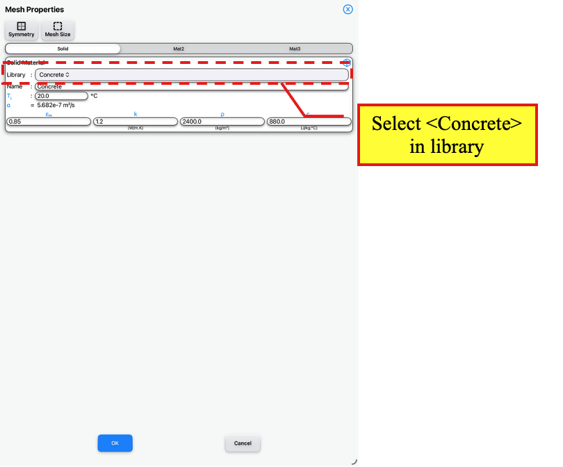
Mesh Properties Page
Under <Solid>, select <Concrete> under library
Next, change the following thermal properties for the concrete material:
εm: 0.7
k: 1.0 in W/m.K
cp: 1000 in J/kg.K
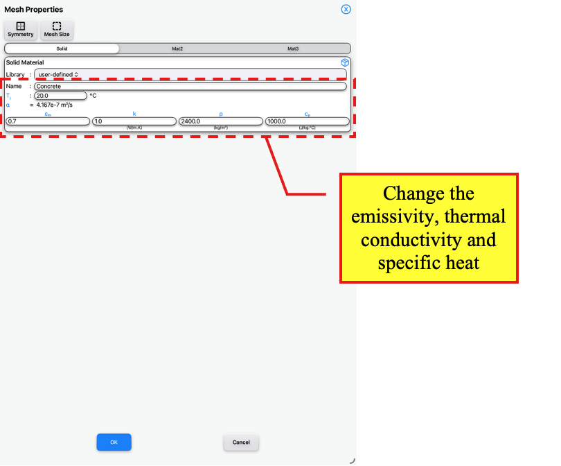
Mesh Properties Page
Change thermal properties for Solid
Then, select <Mat2> and select <Steel> under library. The pre-defined steel thermal properties will be applied to the reinforcement bar.
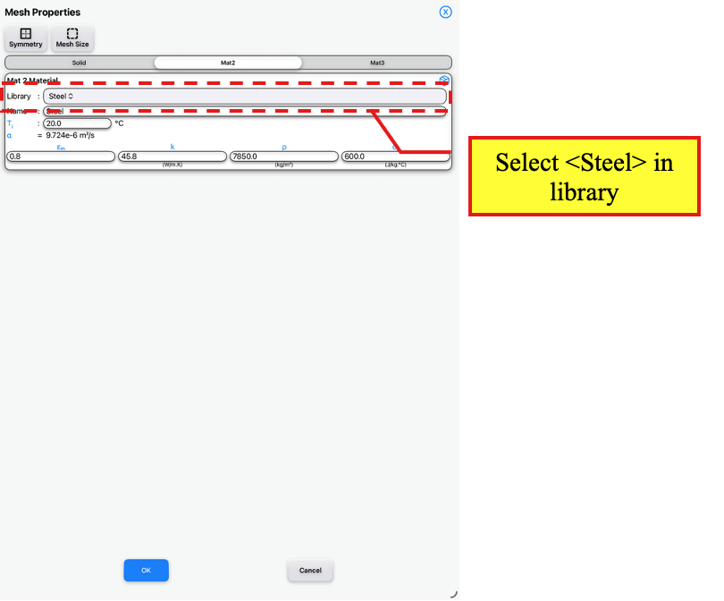
Mesh Properties Page
Under <Mat2>, select <Steel> under library
Next, change the following thermal properties for the steel material:
εm: 0.7
k: 45 in W/m.K
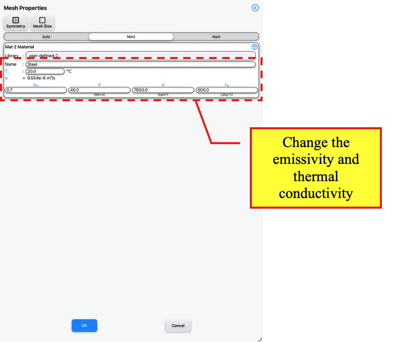
Mesh Properties Page
Change thermal properties for Mat2
Tap the OK button to return to the Thermal Page.
We will then apply the boundary conditions to the model. On the Thermal Page, toggle off <Pick (Single)>.
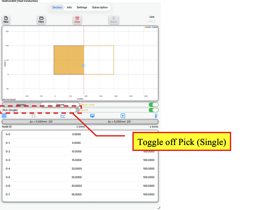
Thermal Page
Toggle off <Pick (Single)>
Next, select a bottom node of the model.
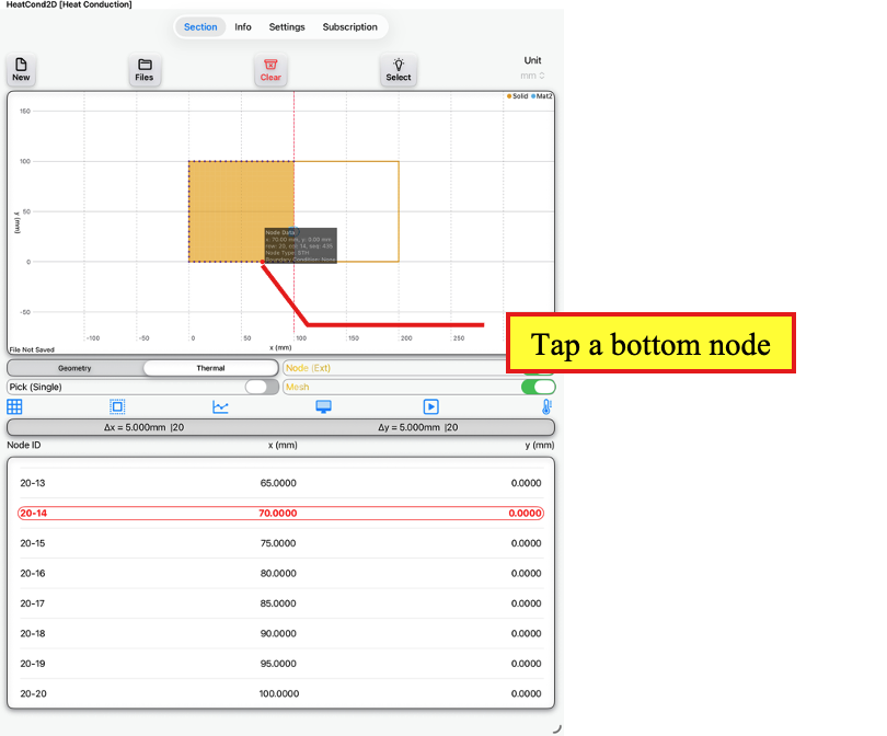
Thermal Page
Tap a bottom node
Then, tap the <Select> button which will bring up a dialog box to confirm if selection is to include end nodes. Tap the Yes button to include the end nodes.
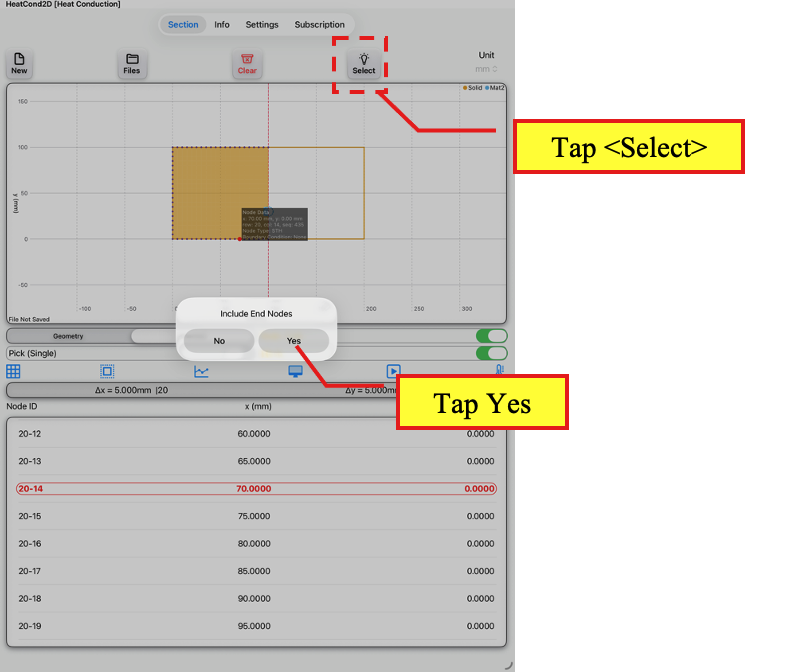
Thermal Page
Tap <Select>
Tap <Yes> to include end nodes
All the bottom nodes on the same plane as the selected node will be highlighted. Next, tap on the Boundary Condition button to access the Node Boundary Conditions Page.
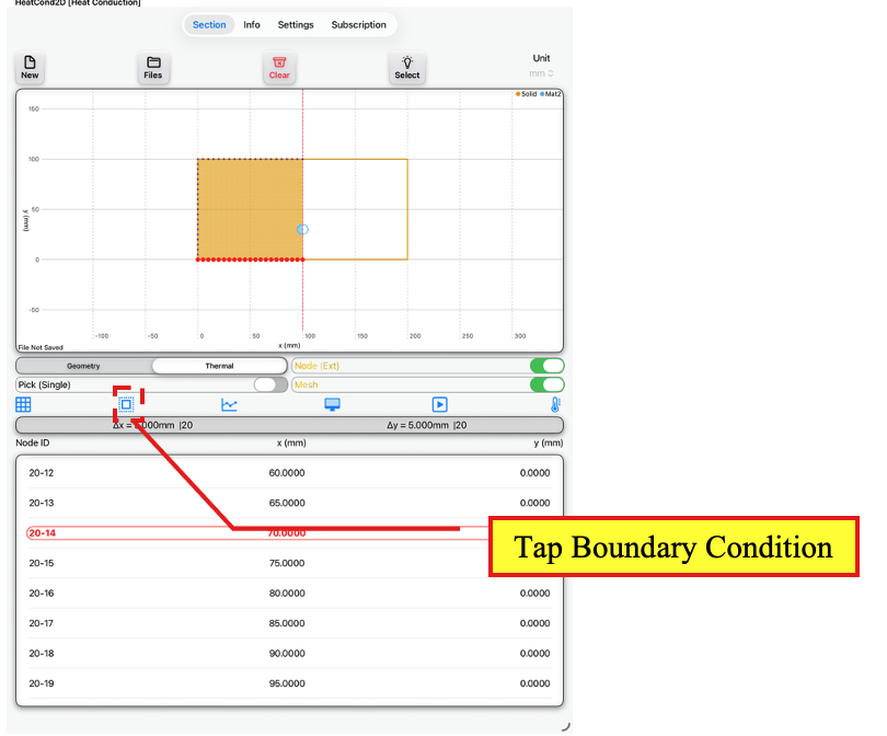
Thermal Page
Tap Boundary Condition button
On the Node Boundary Conditions Page,
Under Exposure Type: Select <Exposure Temp.>
Under Temp. Type: Select <Profile Temp.>
Tap ‘Radiation Gain* (Transient only)’.
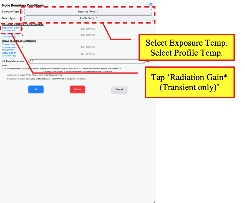
Node Boundary Conditions Page
Select <Exposure Temp.>
Select <Profile Temp.>
Tap ‘Radiation Gain* (Transient only)‘
Enter a View Factor of 1 and Emissivity of 1.0. Then, tap the OK button.
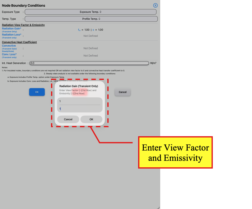
Node Boundary Conditions Page
Enter values for View Factor and Emissivity
Next, tap ‘Convective (Transient Gain/SteadyState)’.
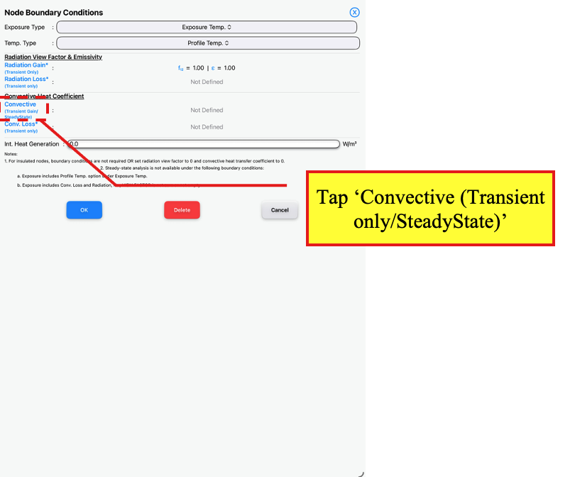
Node Boundary Conditions Page
Tap ‘Convective (Transient only/SteadyState)‘
Enter a Convective Heat Coefficient of 25 W/m².K. Tap the OK button the apply the boundary condition and return to the Thermal Page.
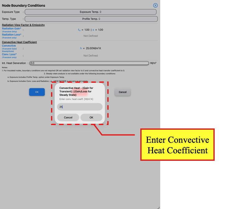
Node Boundary Conditions Page
Enter value for Convective Heat Coefficient
On the Thermal Page, select a top node on the model.
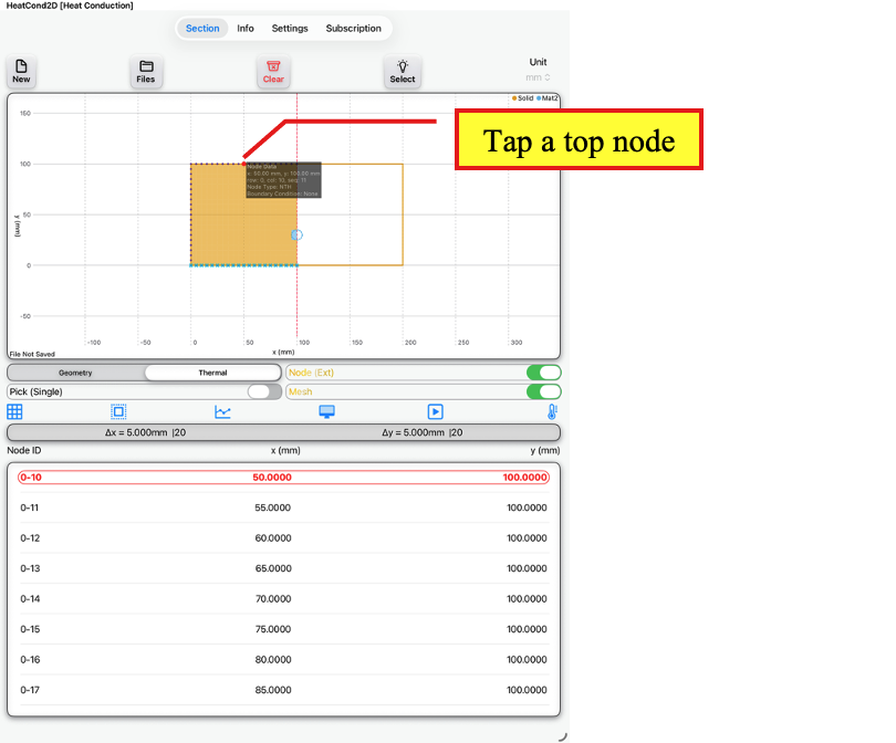
Thermal Page
Tap a top node
Then, tap the <Select> button which will bring up a dialog box to confirm if selection is to include end nodes. Tap the Yes button to include the end nodes.
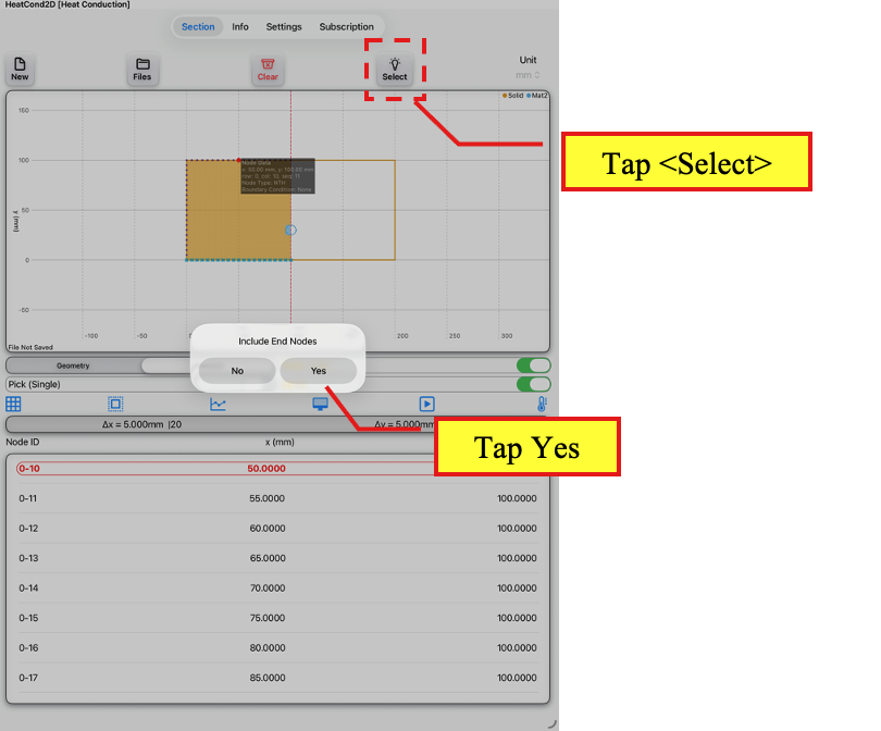
Thermal Page
Tap <Select>
Tap <Yes> to include end nodes
All the bottom nodes on the same plane as the selected node will be highlighted. Next, tap on the Boundary Condition button to access the Node Boundary Conditions Page.
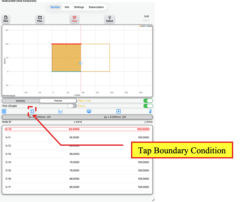
Thermal Page
Tap Boundary Condition button
On the Node Boundary Conditions Page,
Under Exposure Type: Select <Exposure Temp.>
Under Temp. Type: Select <Constant Temp.>
Tap ‘Radiation Loss* (Transient only)’.
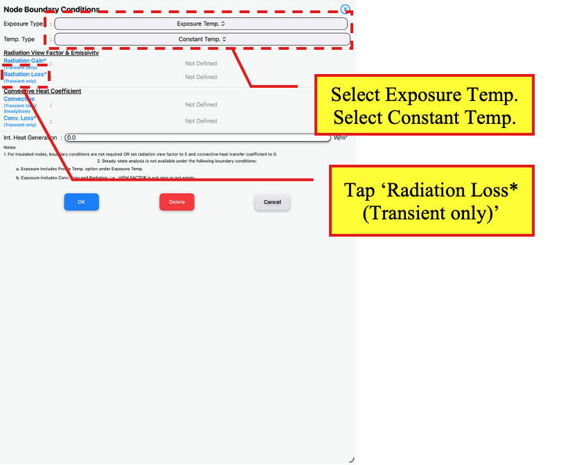
Node Boundary Conditions Page
Select <Exposure Temp.>
Select <Constant Temp.>
Tap ‘Radiation Loss* (Transient only)‘
Enter a View Factor of 1 and Emissivity of 1.0. Then, tap the OK button.
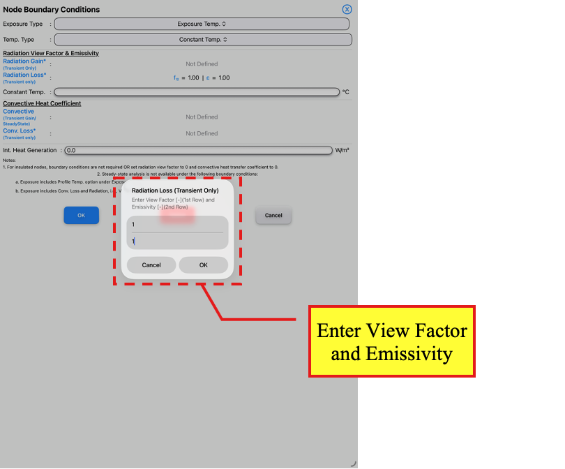
Node Boundary Conditions Page
Enter values for View Factor and Emissivity
Next, tap ‘Conv. Loss* (Transient only)’.
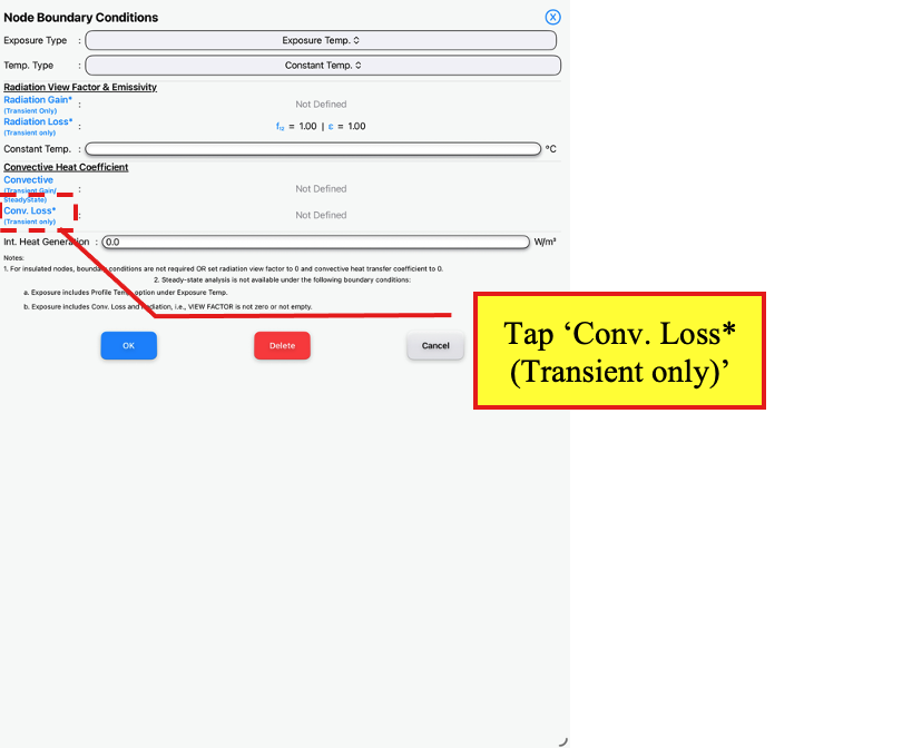
Node Boundary Conditions Page
Tap ‘Conv. Loss* (Transient only)‘
Enter a Convective Heat Coefficient of 4 W/m².K.
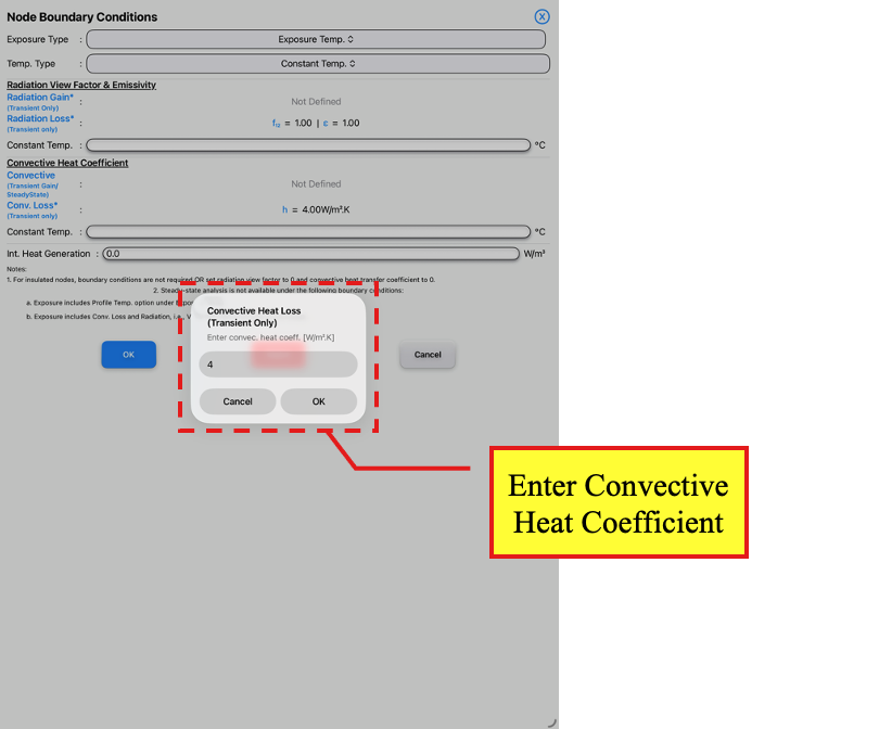
Node Boundary Conditions Page
Enter value for Convective Heat Coefficient
Then, enter a constant temperature of 20°C under each of the Radiation and Convective parts.
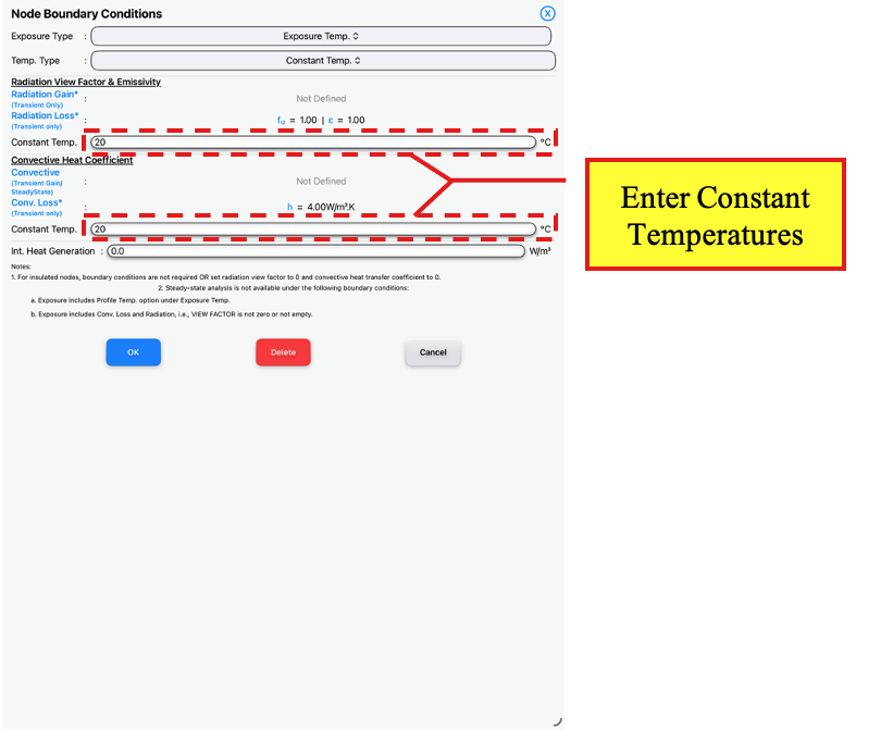
Node Boundary Conditions Page
Enter values for Constant Temperatures
Tap the OK button the apply the boundary condition and return to the Thermal Page. Tap <Clear> to clear the node selection on the Thermal Page.
Note that the external nodes with boundary condition applied will be marked.
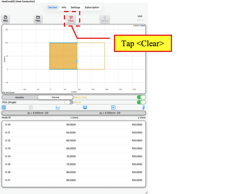
Thermal Page
Tap <Clear>
On the Thermal Page, to view the boundary condition applied to a node, tap on the node.
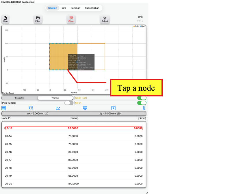
Thermal Page
Tap a node to view node data
Next, we will specify the profile temperature for the fire. On the Thermal Page, tap the Profile button to access the Exposure Source Page.
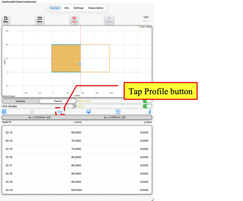
Thermal Page
Tap Profile button
On the Exposure Source Page, tap the Exposure Temperature button to access the Exposure Temperature Page.
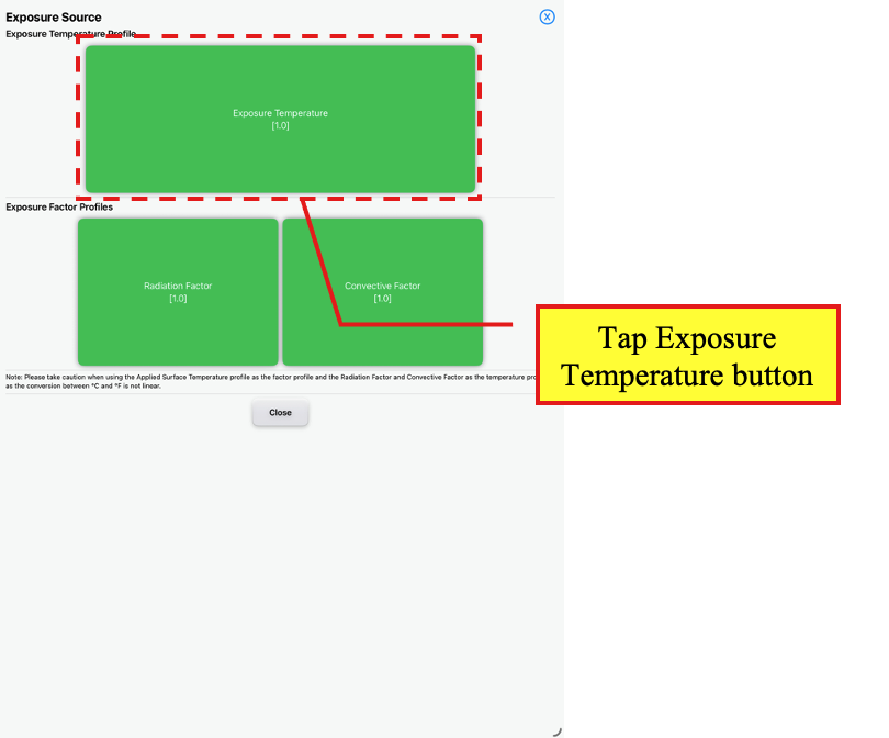
Exposure Source Page
Tap Exposure Temperature button
On the Exposure Temperature Page, tap <Expr> to access the Temperature Expression Page.
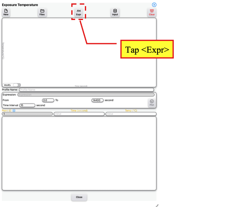
Exposure Temperature Page
Tap <Expr>
On the Temperature Expression Page, select <ISO 834> under Predefined.
Tap the OK button to return to the Exposure Temperature Page.
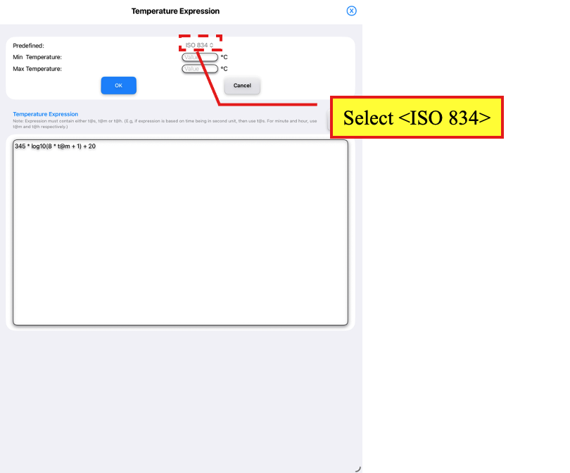
Temperature Expression Page
Select <ISO 834> under Predefined
On the Exposure Temperature Page, tap <Plot> to plot the expression according to the time limits and interval.
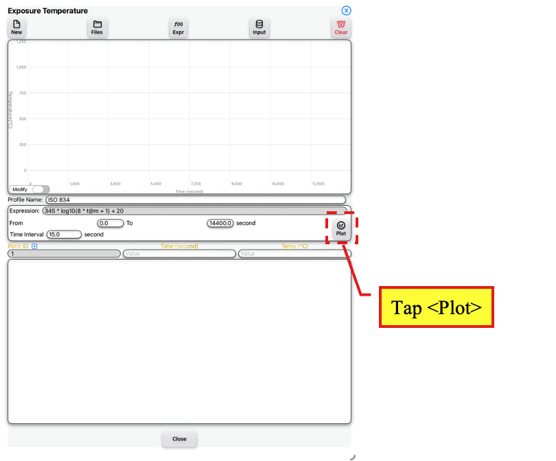
Exposure Temperature Page
Tap <Plot> to plot expression
Tap the OK button when a dialog box appears requesting for confirmation to continue with the plotting.
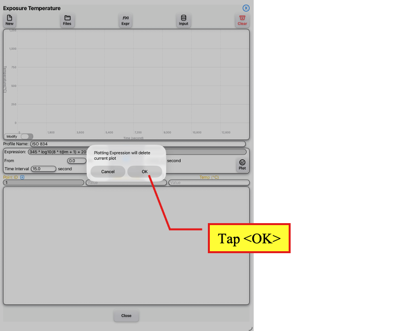
Exposure Temperature Page
Tap <OK> to continue plotting
Tap the Close button to return to the Exposure Source Page.
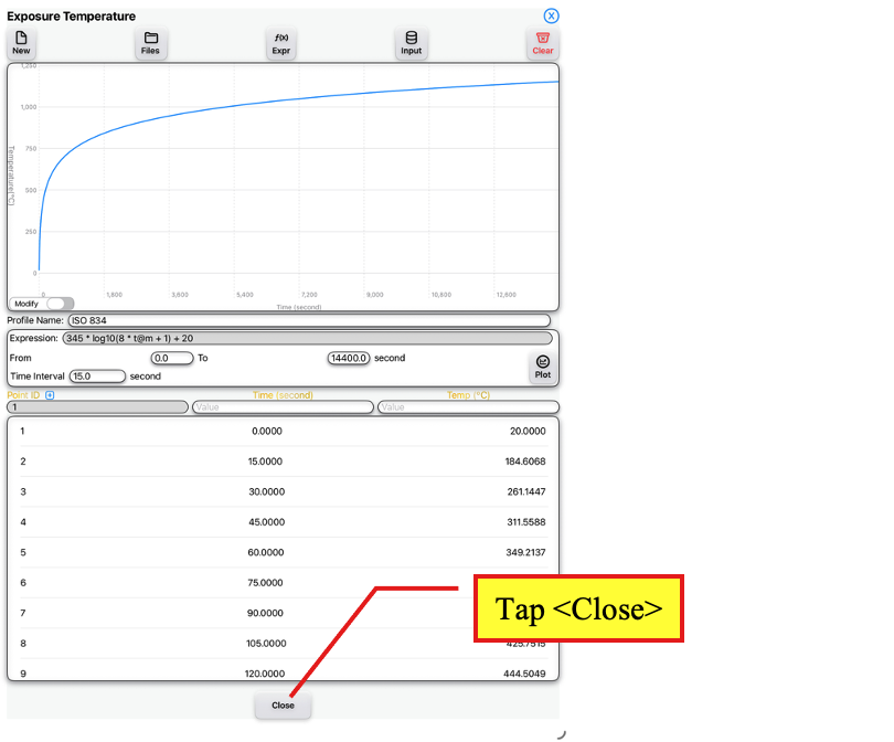
Exposure Temperature Page
Tap <Close>
On the Exposure Source Page, tap the Close button to return to the Thermal Page.
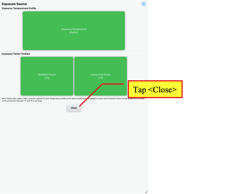
Exposure Source Page
Tap <Close>
On the Thermal page, tap the Simulation Data button to access the Simulation Data Page.
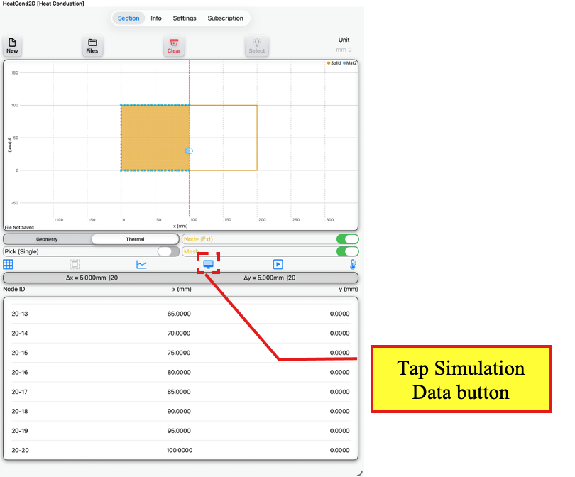
Thermal Page
Tap Simulation Data button
On the Simulation Data Page, under Solver select Transient.
Enter a run time of 5400 seconds and Δt of 0.5 second. When using the transient solver, check that under each material (i.e., S1 for Solid and M2 for Mat2) that there are no red ticks under the Stability Check.
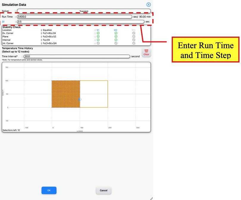
Simulation Data Page
Enter Run Time and Time Step
Tap the OK button to apply to simulation data and return to the Thermal Page.
On the Thermal Page, tap the Run button to run the heat transfer analysis.
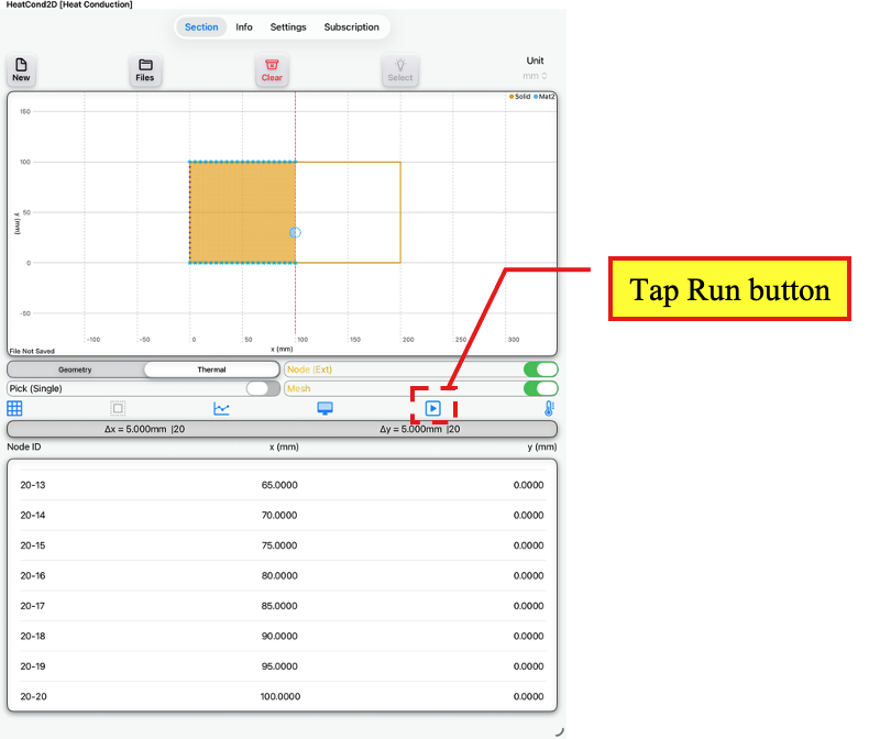
Thermal Page
Tap Run button
A dialog box will appear. Take the OK button to continue the analysis.
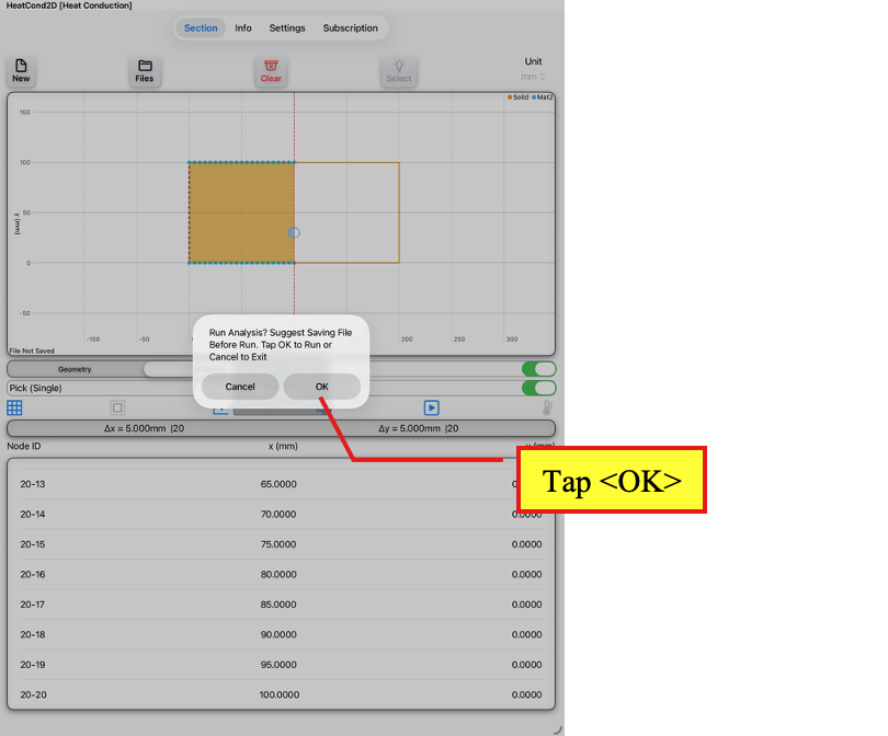
Thermal Page
Tap <OK> to run analysis when dialog box appears
The Results Page will automatically appear after the analysis has been completed.
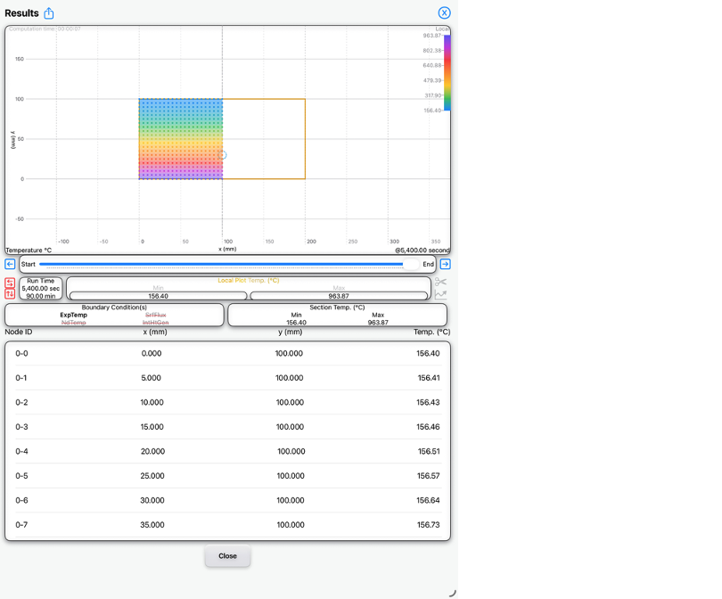
Results Page
Observe results
On the Results Page, tap on the node at the centre of the reinforcement bar at coordinates (100 mm, 30 mm). Tap the Time-History button (with ‘1’ showing) to view the time-history for that node.
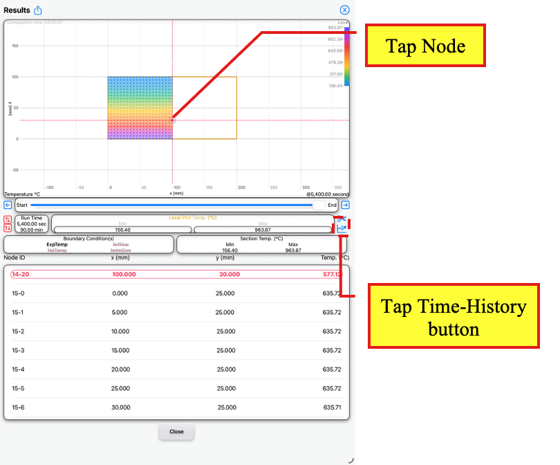
Results Page
Tap node
Tap Time-History button
On the Time History Plot Page, tap the Add button to add this node to the time-history plot list and tap close to return to the Results Page.
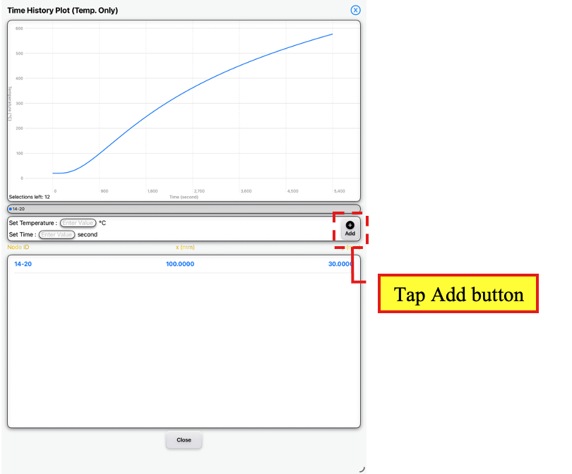
Time History Plot Page
Tap <Add>
Back on the Results Page, tap on the node located to the left hand side of the model at coordinates (0 mm, 30 mm). Tap the Time-History button (with ‘1’ showing) to view the time-history for that node.
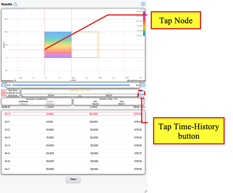
Results Page
Tap node
Tap Time-History button
On the Time History Plot Page, tap the Add button to add this node to the time-history plot list and tap close to return to the Results Page.
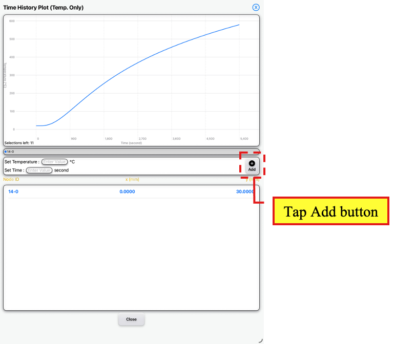
Time History Plot Page
Tap <Add>
To view the Time History Plots for all the selected nodes, unselect any node on the Results Page.
Then, tap the Time-History button (without ‘1’ showing).
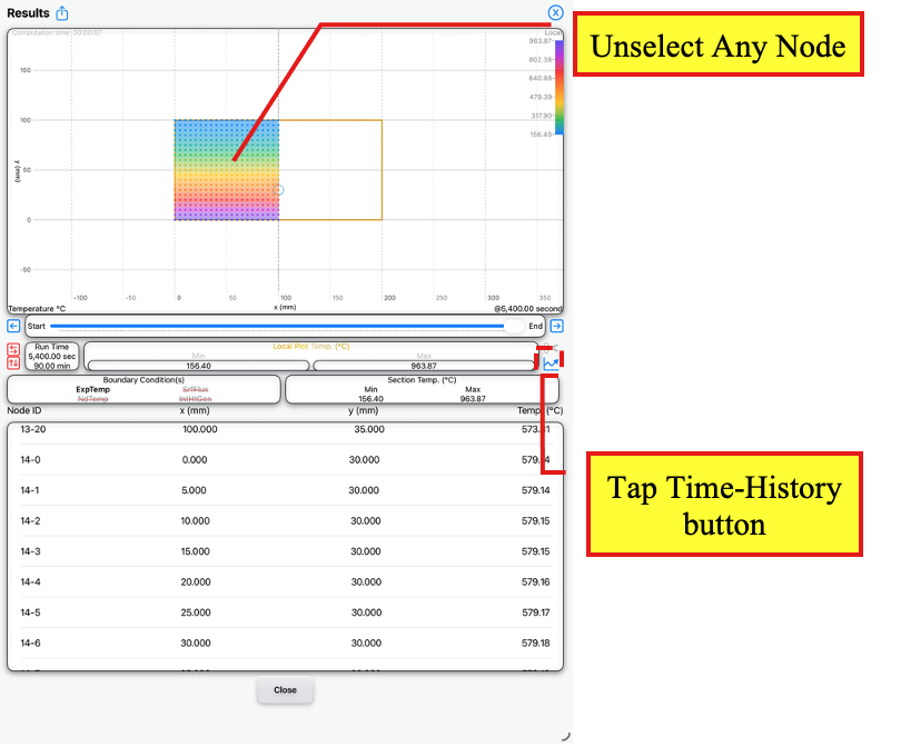
Results Page
Unselect any selected node
Tap Time-History button
On the Time-History Plot Page, tap <Select All>.
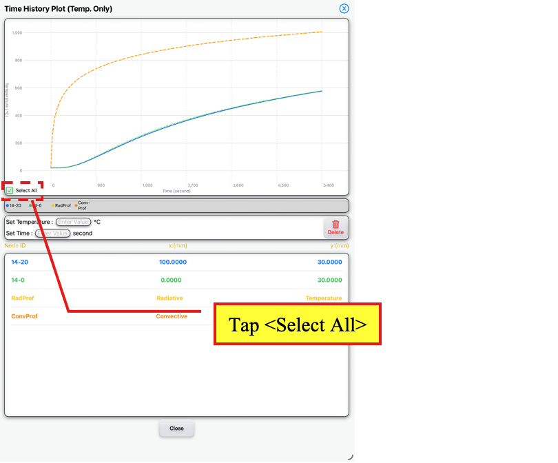
Time History Plot Page
Tap <Select All>
Based on the time-history plots, the following temperatures at these times are observed at time of 5,400 seconds.
Concrete temperature at coordinates (0 mm, 30 mm): 579.14°C (Node ID 14-0)
Reinforcement bar at coordinates (100 mm, 30 mm): 577.12°C (Node ID 14-20)
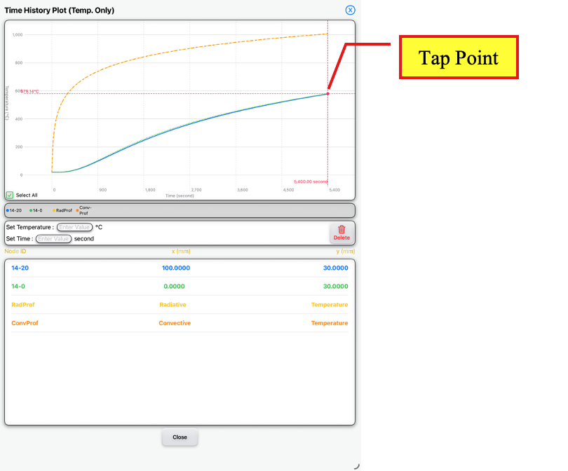
Time History Plot Page
Tap a point
Tap the Close button to return to the Results Page.
On the Results Page, tap a top node on the model and tap the <Slice> button to cut horizontal and vertical temperature slices through the node on the Section Slices Page.
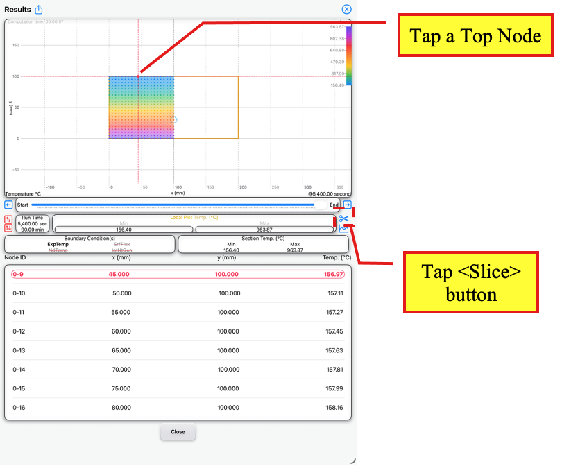
Results Page
Tap a top node
Tap <Slice>
On the Section Slices Page, observe that the temperatures at the top of the slab is between 156.4°C to 158.52°C.
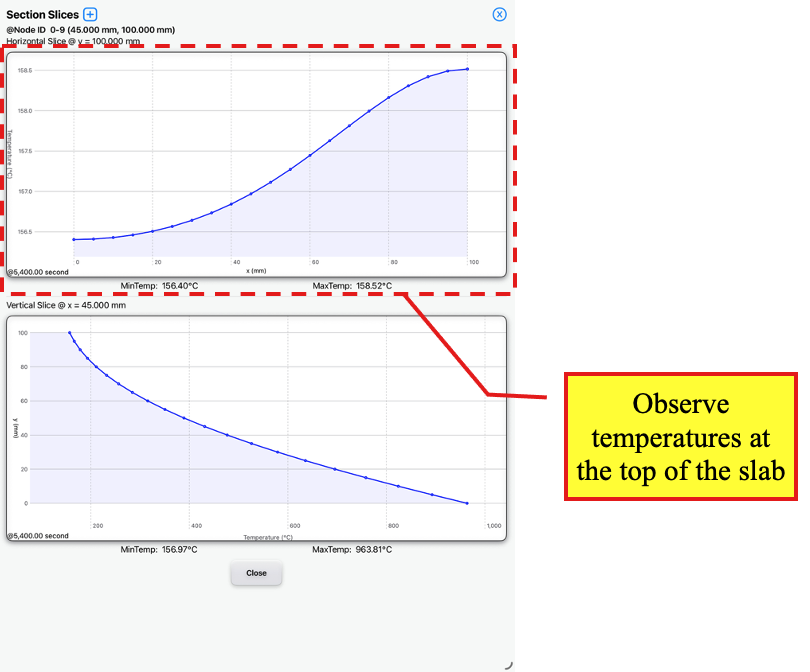
Section Slices Page
Observe temperatures
Based on the heat transfer analysis, we can summarise that for this example, the inclusion of the reinforcement bar in the model affects the temperature of the concrete by approximately 2°C and the heat transfer analysis with the assumed design parameters estimates the reinforcement temperature at 577°C.
For comparison, the reinforcement bar limiting temperature is typically between 500°C to 600°C depending on the action that the slab is required to carry under a fire scenario.
In addition, the non-fire exposed side of the top of the slab is between 156.4°C to 158.52°C resulting in a temperature rise of 136.4°C to 138.52°C (given the initial slab temperature is 20°C), which is less than the maximum average temperature rise for insulation of 140°C.
Note that this heat analysis is only an example and must not be applied to actual design with similar slab and reinforcement arrangement without review and approval of a qualified structural and fire engineer.