Modelling Multi-Layer House Wall Insulation
In this first article, we will analyse the heat transfer of a multi-layer residential composite wall.
The original problem, sourced from an online lecture on thermal resistance [video link here, please note that you will be leaving our website. We are not responsible for the content or safety of external sites.] by Dr. Ron Hugo is modelled using the HeatCond2D app to compare its numerical solution against the analytical solution.
Problem Definitions and Assumptions
The wall geometry and boundary conditions are illustrated in the sketch below.
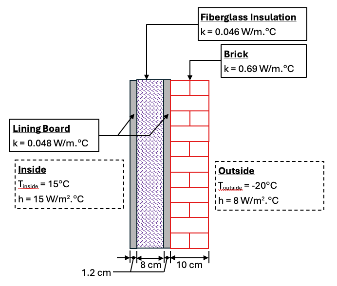
Sketch
Wall Arrangement
Based on the physical arrangement and exposure conditions, the heat transfer process can be modelled as steady-state and one-dimensional under the following assumptions:
Uniform Convection: Convective heat transfer is applied uniformly across both external surfaces.
One-Dimensional Flow: Temperature gradients and heat flux in the vertical and depth directions are negligible.
Steady-State Conditions: The system represents long-term, steady-state heat loss per unit area after initial transient effects have dissipated.
[Tips & Tricks: By observing the boundary conditions, which is the temperature on each side wall, we can tell that the heat will flow from the inside to the outside, i.e., from high temperature to low temperature.]
Numerical Procedure and Results
(Detailed modelling steps are provided at the end of this article.)
Following the analysis using HeatCond2D, the surface temperatures and heat conduction flux are evaluated on the Results Page of the app:
Indoor Surface Temperature (Lining Board): 14.1°C
Outdoor Surface Temperature (Brick wall): -18.3°C
Conduction heat flux: Constant heat flux of 13.59 W/m² along the x-axis.
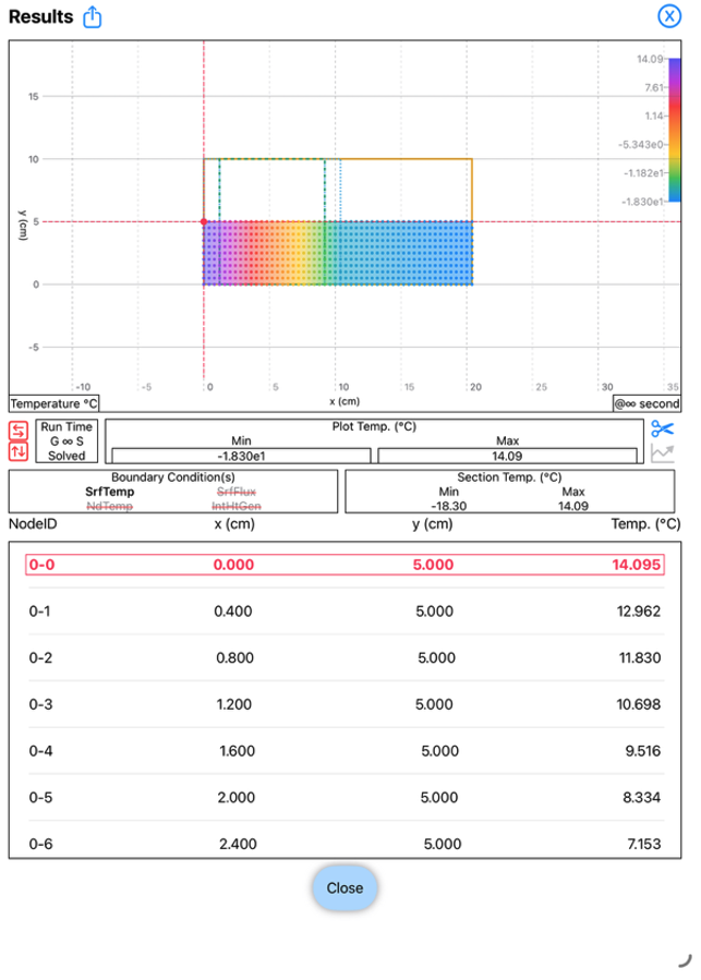
HeatCond2D Results Page
Temperature at surface of Lining Board
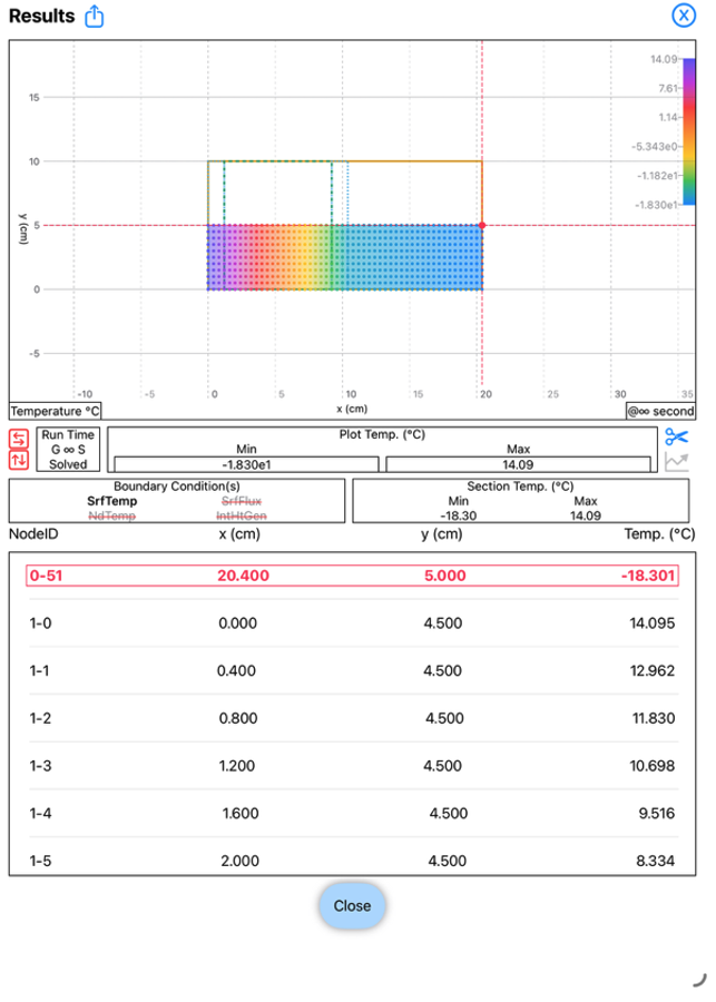
HeatCond2D Results Page
Temperature at surface of Brick wall
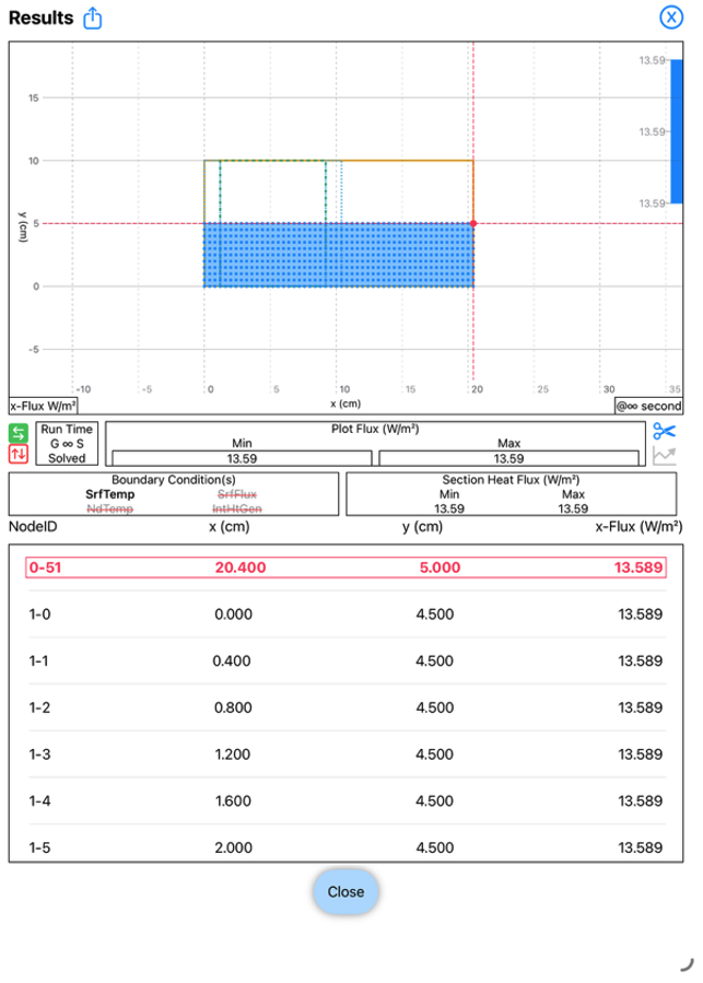
HeatCond2D Results Page
Conduction heat flux through the composite wall
The analytical solution from the online lecture gives a heat loss rate of 13.59 W/m², which perfectly aligns with the heat flux estimated from HeatCond2D.
The .txt input file for the HeatCond2D model is available for download here.
If you have any queries or feedback regarding this article, please contact us.
If you wish to download HeatCond2D, click here.
Step-by-Step Modelling Procedure
Please note that while the step-by-step procedure may look tedious at first, the modelling process will become quick and efficient once you get used to the app workflow.
Our first step is to create the wall section.
Open the HeatCond2D app and tap on the Section Page. Tap <Solid> to ensure that the Solid Element is selected. We will treat the wall section as the Solid Element as this is the base building element for the app.
[Tips & Tricks: To save time when creating a section, utilise the built-in Section and Shape Templates and adjust the creation to suit your section.]
Next tap on the Section Template button to access the Section Template Page.
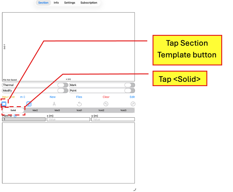
Section Page
Tap <Solid>
Tap Section Template button
In the Section Template Page, tap the Rectangular Section button to bring up the template for a rectangular section.
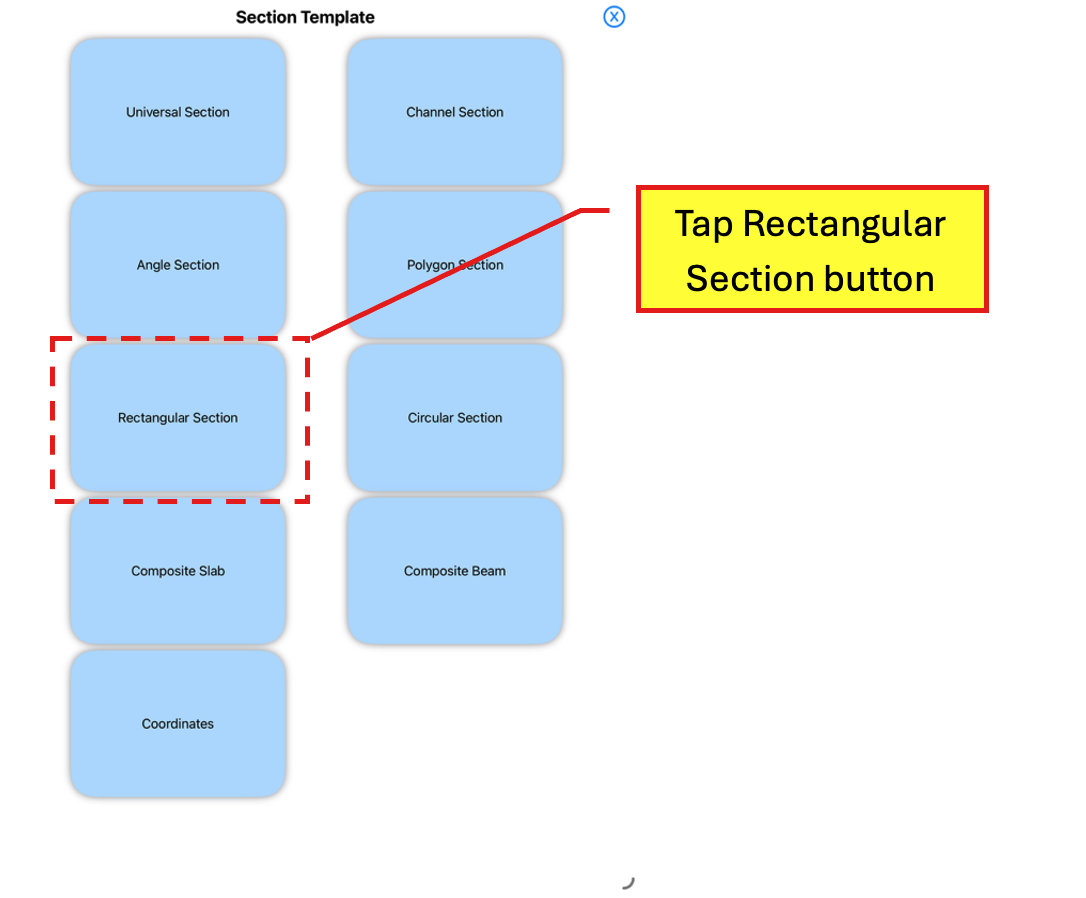
Section Template
Tap Rectangular Section button
Under Input Unit, select cm from the drop down list to change the unit. Then enter the following dimensions:
b0 = 20.4 in cm
d0 = 10 in cm
Leave b1 and d1 empty.
Ensure that the Outer Element is set to Solid and Inner Element is set to Void1.
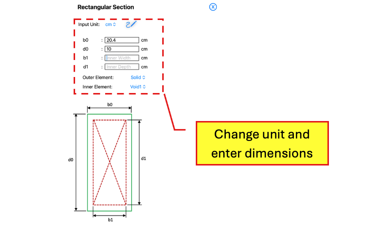
Rectangular Section (Template)
Change unit and enter dimensions
Tap on the Scribble button to create the rectangular section.
Back in the Section Page, tap on <Mat2> to select the Mat2 element.
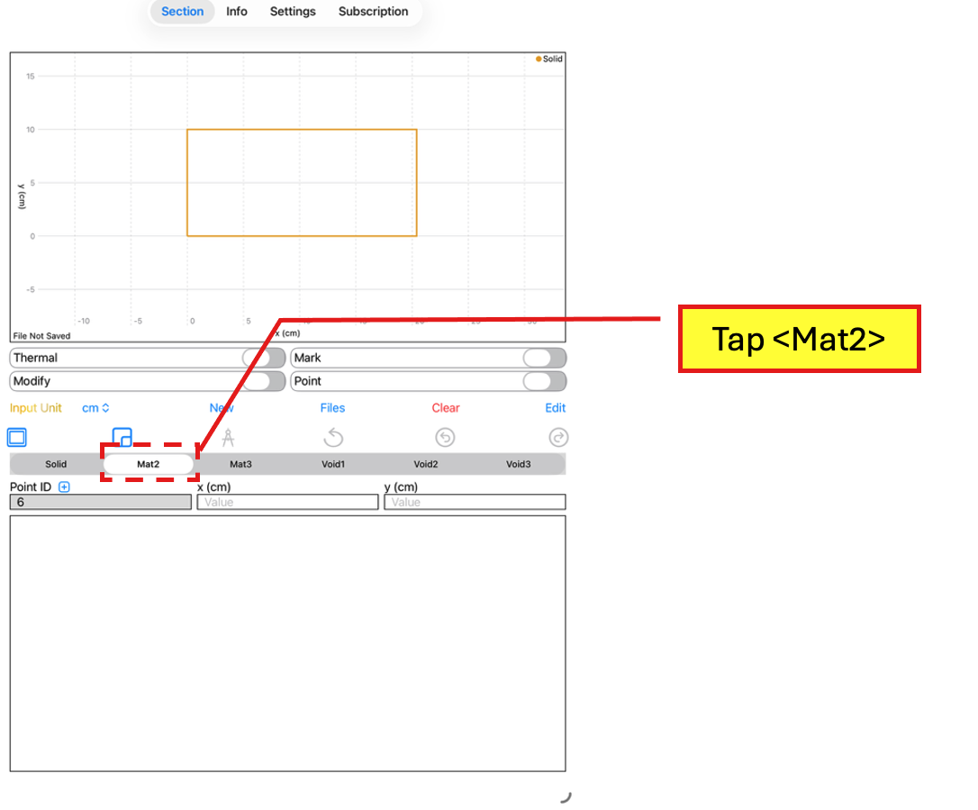
Section Page
Tap <Mat2>
Next we will create the Lining Boards as Mat2 elements. As we will be using the Mat2 element for two lining boards that are separated by the Fiberboard Insulation, we will manually enter the coordinates for the Lining Boards.
Under the x and y fields, enter 0 and 0 as Point ID 6 and tap the “+” button followed by the remaining coordinates, tapping the “+” button each time.
Point ID 7: 10.4, 0
Point ID 8: 10.4, 10
Point ID 9: 9.2, 10
Point ID 10: 9.2, 0
Point ID 11: 1.2, 0
Point ID 12: 1.2, 10
Point ID 13: 0, 10
Point ID 14: 0, 0 to close the element.
After creating the Mat2 element, tap on <Mat3> which will be used for the Fibreglass Insulation. Tap on the Shape Template button to access the Shape Template Page.
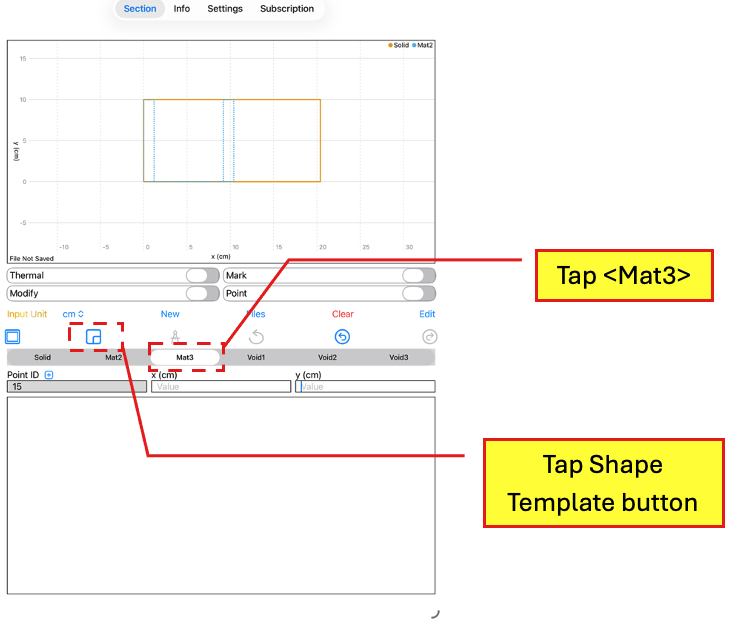
Section Page
Tap <Mat3>
Tap Shape Template button
Select <Rectangle> and enter the following information:
cx = 5.2 in cm
cy = 5 in cm
b0 = 8 in cm
d0 = 10 in cm
Leave t empty.
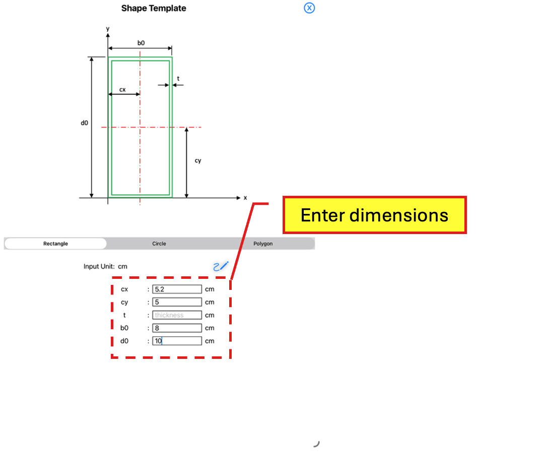
Shape Template
Tap <Rectangle>
Enter dimensions
Tap on the Scribble button to create the rectangle.
Next, in the Section Page, toggle on the Thermal toggle button to access the Thermal Page.
We will then generate the meshes for the model.
Tap on the Mesh Properties button to access the Mesh Properties Page.
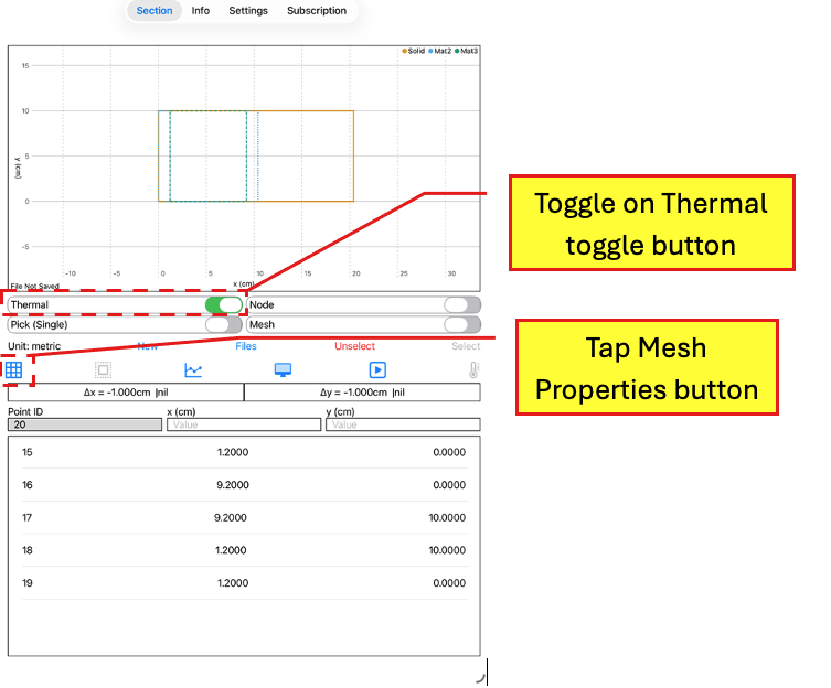
Section Page -> Thermal Page
Toggle on Thermal toggle button
Tap Mesh Properties button
[Tips & Tricks: When developing models, leverage symmetry wherever applicable to minimise computational demand.]
Tap on the Quad Section button to access the Quad Section Page.
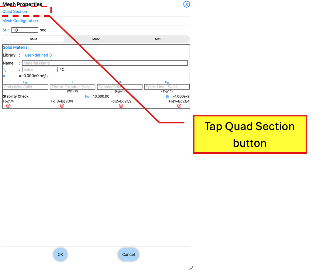
Mesh Properties Page
Tap Quad Section button
In the Quad Section Page, tap the “SouthWest Corner” and “SouthEast Corner” buttons. Tap on the OK button to return to the Mesh Properties Page.
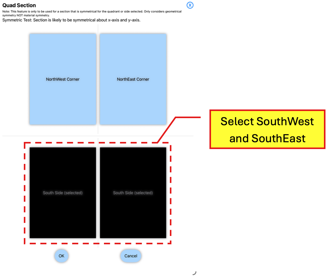
Quad Section Page
Tap SouthWest and SouthEast buttons
In the Mesh Properties Page, tap on the Mesh Configuration button to access the Mesh Configuration button.
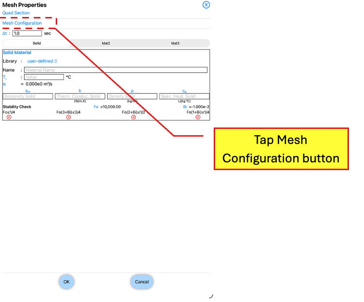
Mesh Properties
Tap Mesh Configuration button
Enter Δx of 0.4 in cm and Δy of 0.5 in cm. Leave Mesh Symmetry as “About y- and x- axes” and Selected Mesh Size as “Modified Mesh Size”.
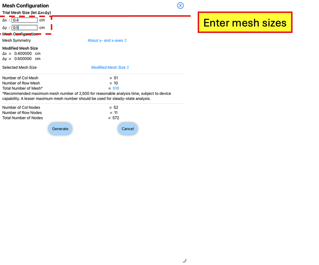
Mesh Configuration Page
Enter mesh sizes
Tap the Generate button to return to the Mesh Properties Page.
[Tips & Tricks: When running a steady-state analysis, the Fo and Bi stability criteria are not required to be met. In addition for steady-state analysis, only the k, thermal conductivity is used in the analysis, therefore other parameters (Ti, εm, ρ and cp) can be set to 1.]
In the Mesh Properties Page, select <Solid> and enter the following information:
Name: Brick
Ti: 1
εm: 1
k: 0.69 in W/m.K
ρ: 1
cp: 1
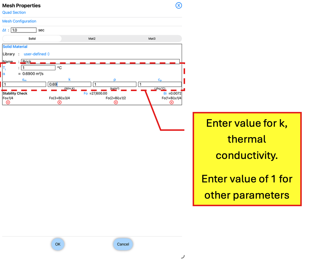
Mesh Properties Page
Under <Solid>, enter value for k and 1 for other parameters
Next, select <Mat2> and enter the following information:
Name: Lining Board
Ti: 1
εm: 1
k: 0.048 in W/m.K
ρ: 1
cp: 1
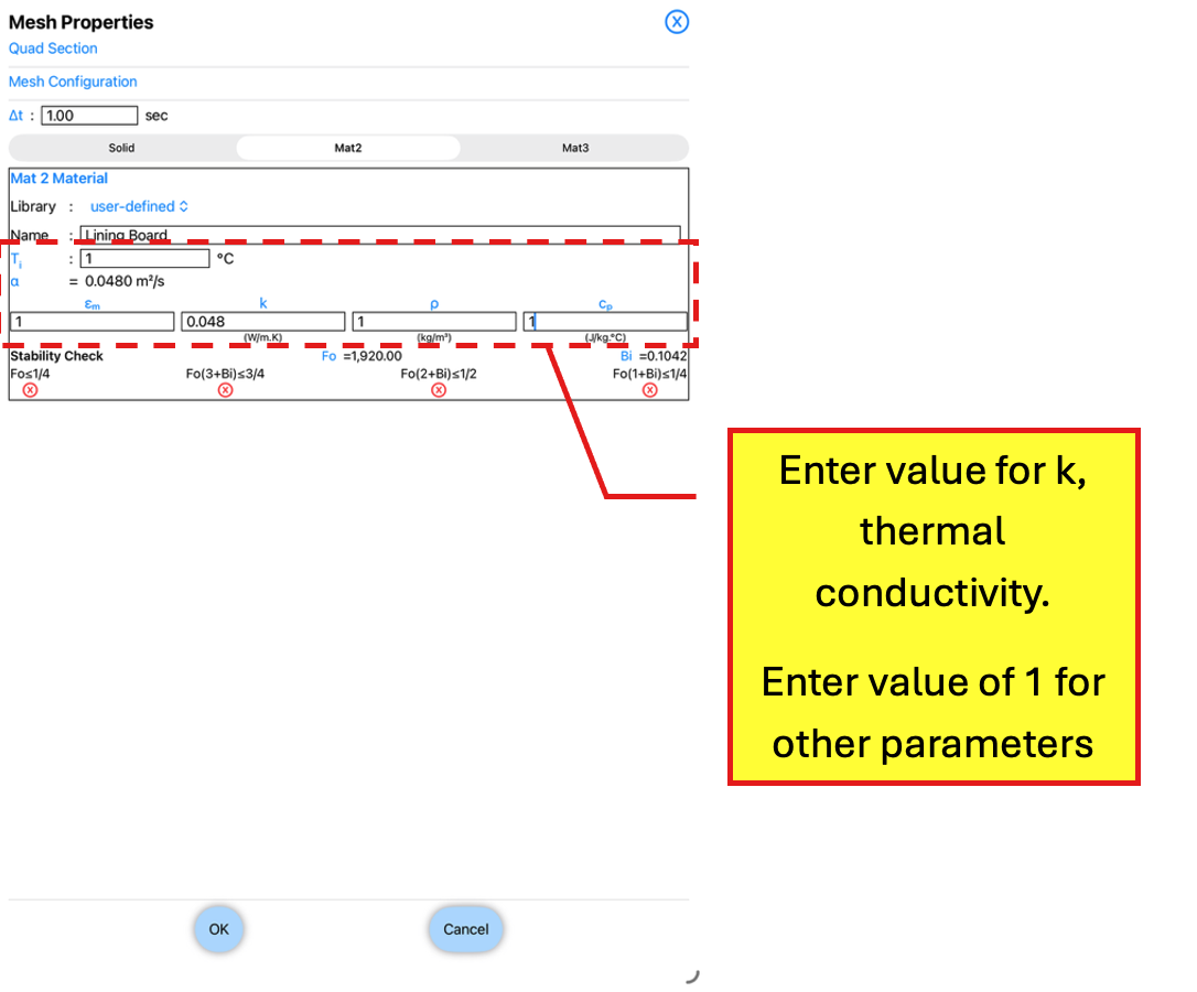
Mesh Properties Page
Under <Mat2>, enter value for k and 1 for other parameters
Finally, select <Mat3> and enter the following information:
Name: Fiberglass Insulation
Ti: 1
εm: 1
k: 0.046 in W/m.K
ρ: 1
cp: 1
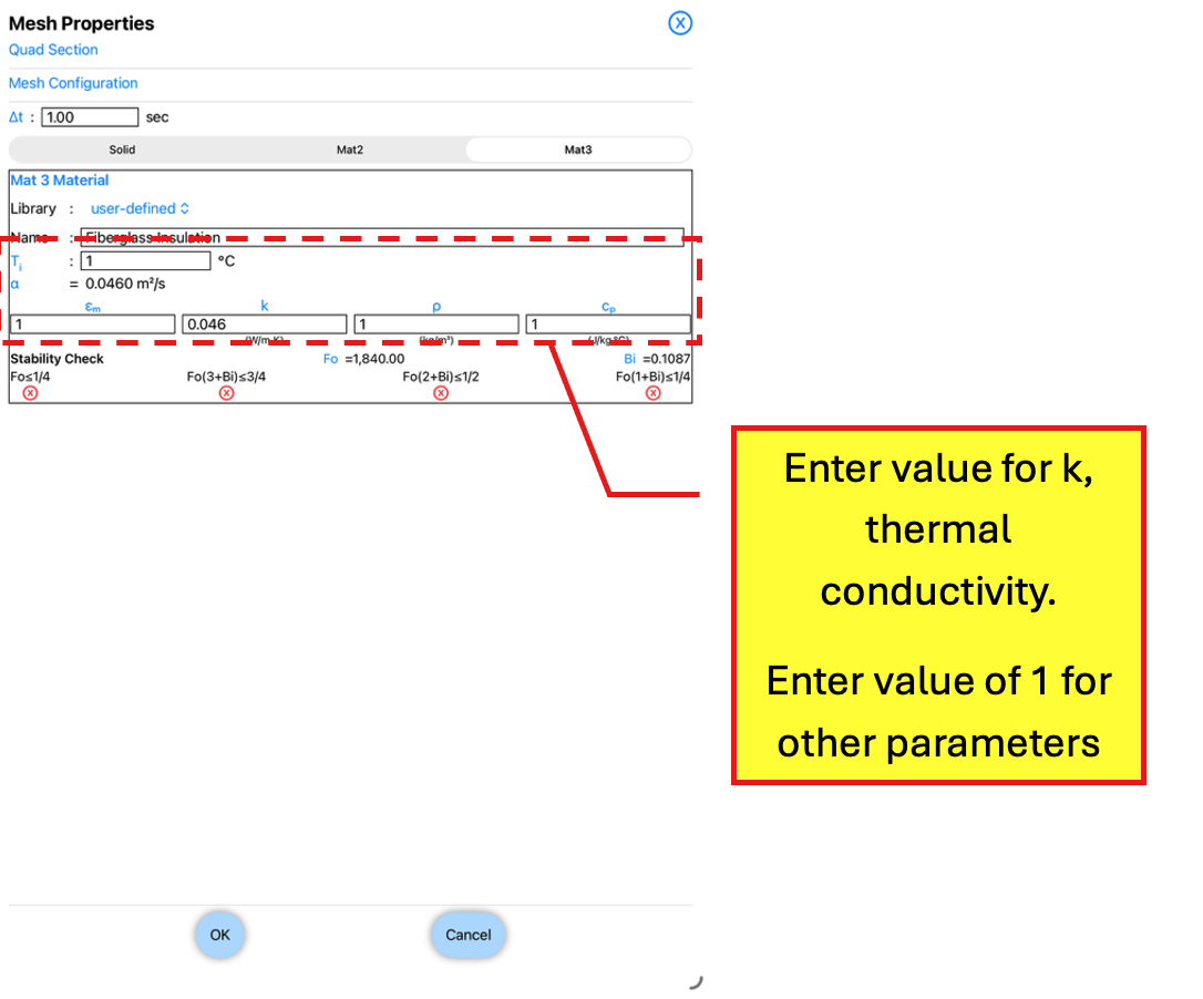
Mesh Properties Page
Under <Mat3>, enter value for k and 1 for other parameters
Tap the OK button to return to the Thermal Page.
We will then apply the boundary conditions to the nodes. Toggle on the Pick (Single) toggle button to show Pick (Group).
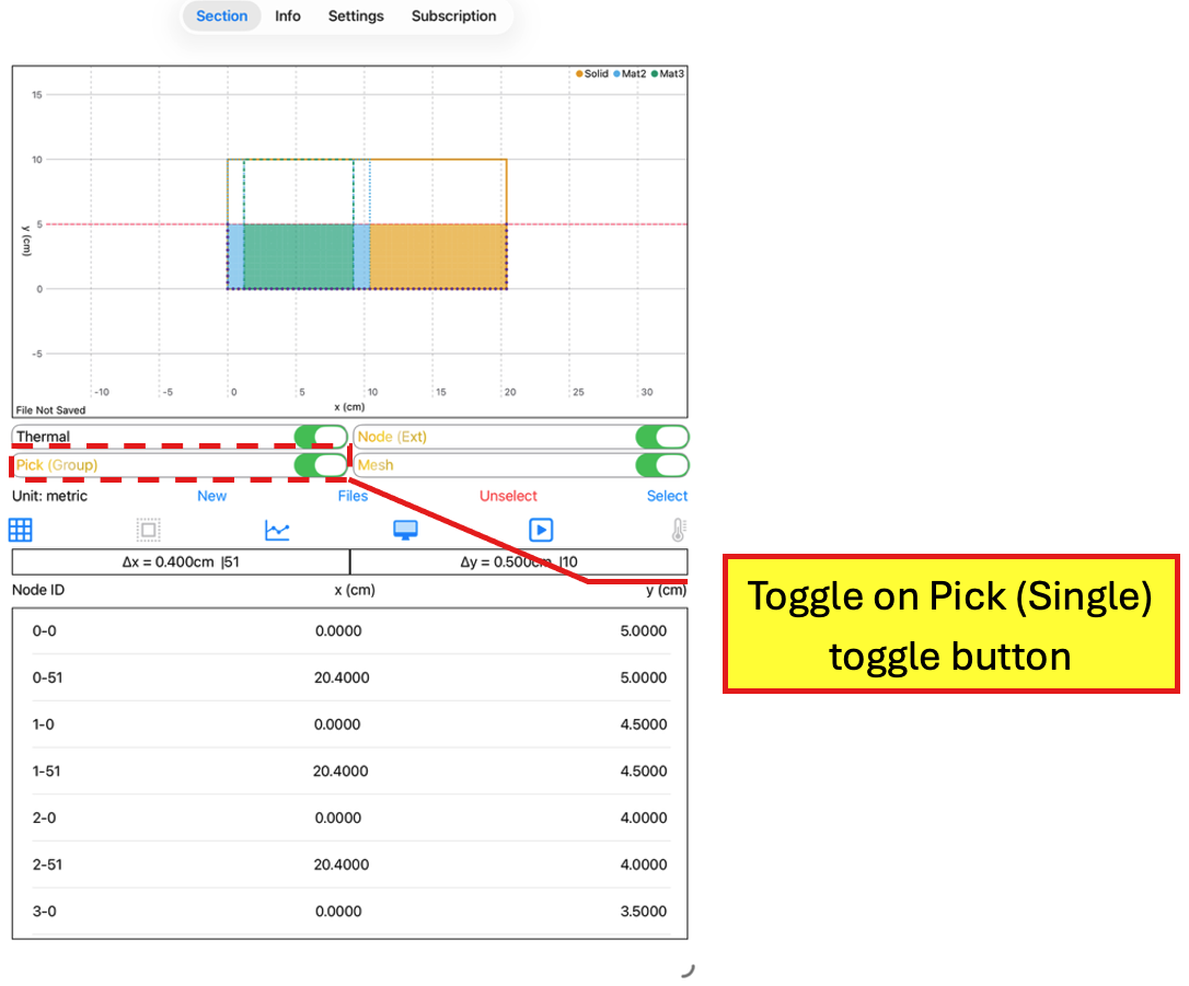
Thermal Page (Thermal Toggle button On)
Toggle on Pick (Single) toggle button
Tap around the left hand side external nodes to create a band. Tap Select to close the band. The selected nodes will be highlighted.
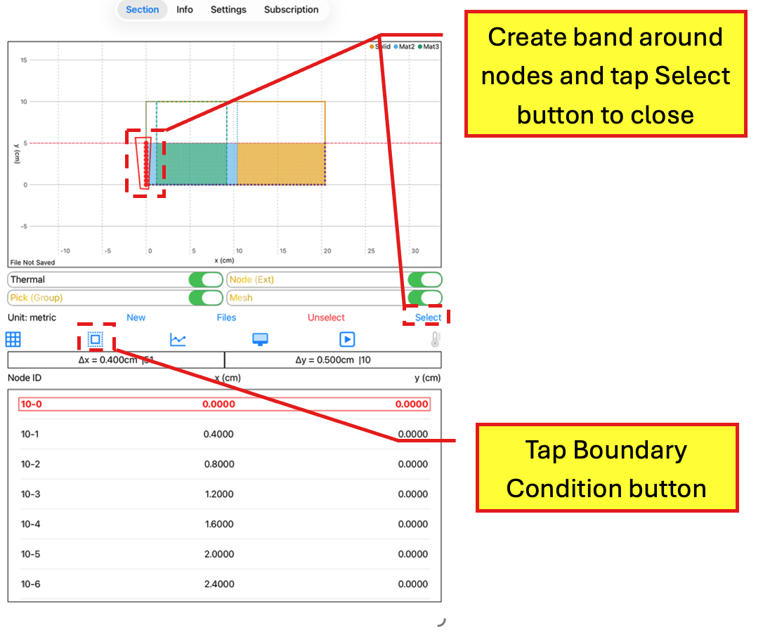
Thermal Page (Thermal Toggle button On)
Create band around left side external nodes
Tap Boundary Condition button
Next tap the Boundary Condition button to access the Node Boundary Conditions Page. Enter the following information:
Select “Surface Temp.“ as the Exposure Type
Select “Constant Temp.” as the Temp. Type
Constant Temp.: 15 in °C
Tap Convective (Transient Gain/SteadyState) and enter h = 15 in W/m^2.K
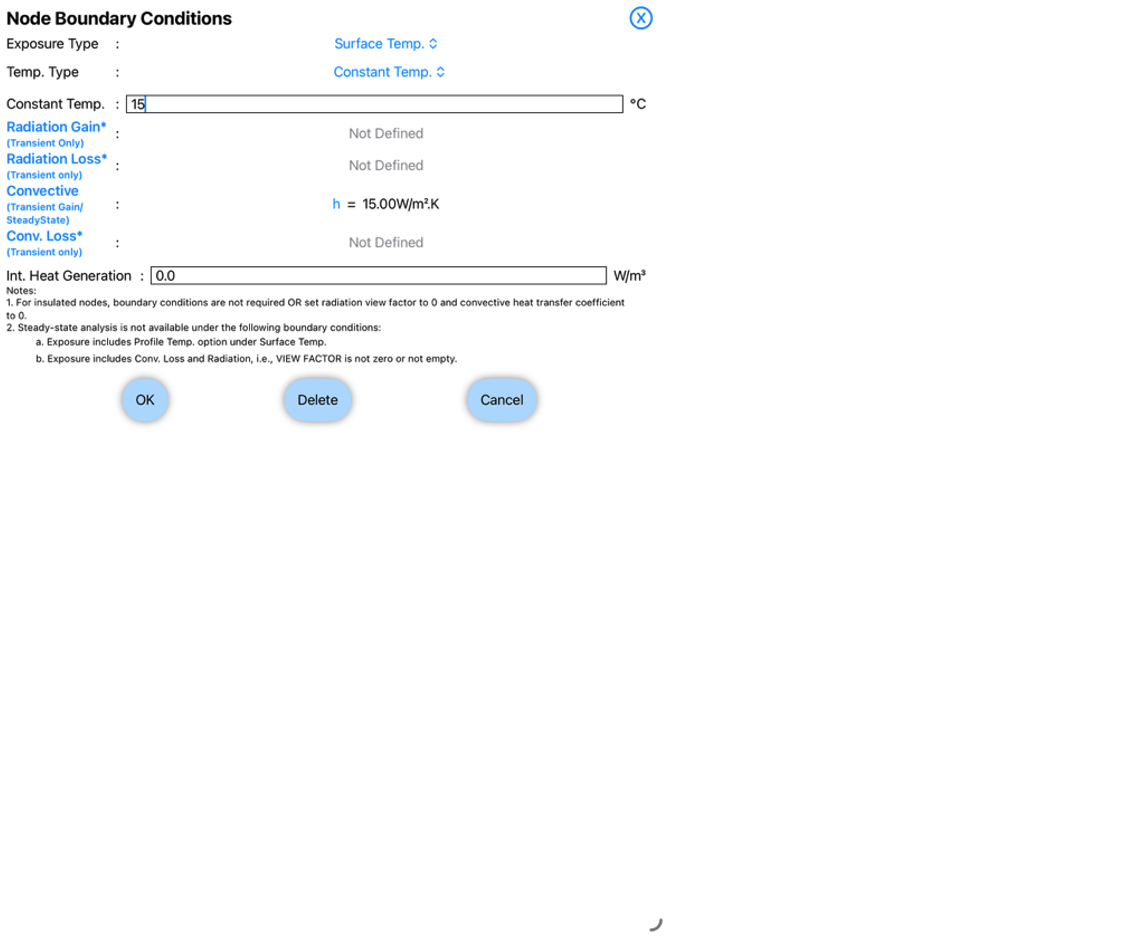
Node Boundary Conditions Page
Enter values for Constant Temp. and Convective (Transient/Steady-State) for left side external nodes
Tap the OK button to return to the Thermal Page.
Back in the Thermal Page, tap around the right hand side external nodes to create a band. Tap Select to close the band. The selected nodes will be highlighted.
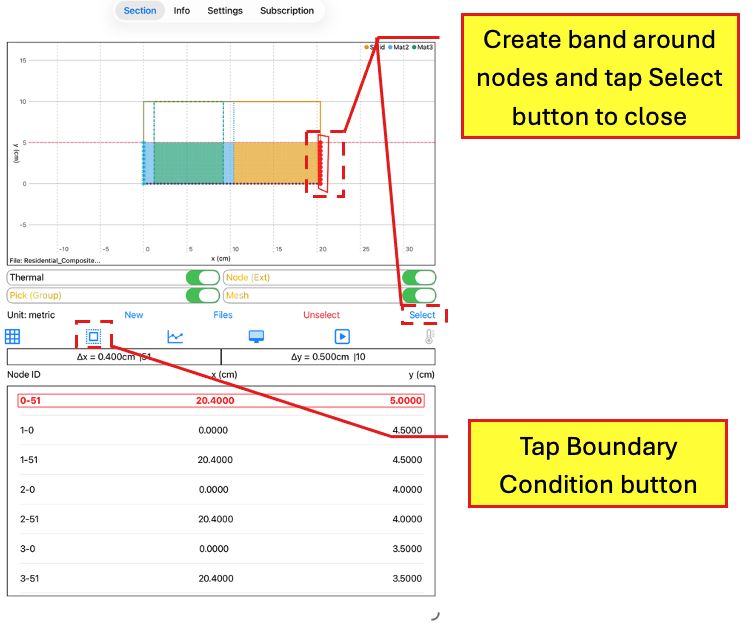
Thermal Page (Thermal Toggle button On)
Create band around right side external nodes
Tap Boundary Condition button
Next tap the Boundary Condition button to access the Node Boundary Conditions Page. Enter the following information:
Select “Surface Temp.“ as the Exposure Type
Select “Constant Temp.” as the Temp. Type
Constant Temp.: -20 in °C
Tap Convective (Transient Gain/SteadyState) and enter h = 8 in W/m^2.K
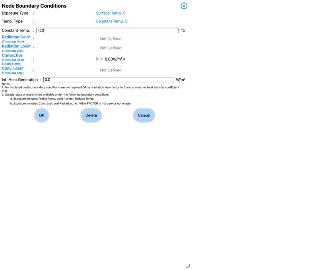
Node Boundary Conditions Page
Enter values for Constant Temp. and Convective (Transient/Steady-State) for right side external nodes
Tap the OK button to return to the Thermal Page.
[Warning: When running a steady-state analysis, note that only one value can be entered for the convective heat transfer coefficient unlike a transient analysis where convective gain and convective loss can have separate values.]
In the Thermal Page, tap an external node to view the node data. Next, tap the Simulation Data button to access the Simulation Data Page.
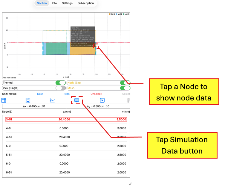
Thermal Page (Thermal Toggle button On)
Tap a Node to show node data
Tap Simulation Data button
In the Simulation Data Page, select <Steady-State> and <Gauss-Seidel>. Tap the OK button to return to the Thermal Page.
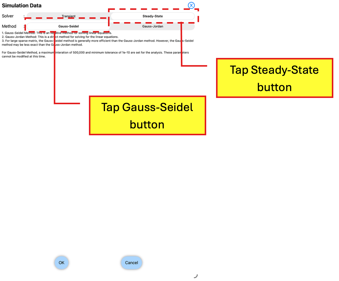
Simulation Data Page
Tap <Steady-State>
Tap <Gauss-Seidel>
In the Thermal Page, tap the Run button to run the heat transfer analysis.
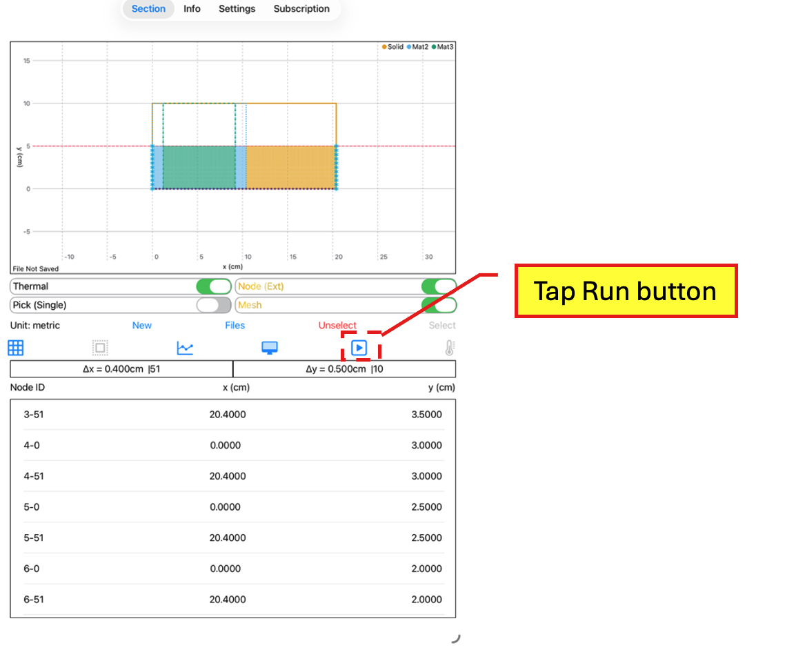
Thermal Page (Thermal Toggle button On)
Tap Run button
A dialog box will appear. Tap the OK button to continue with the analysis.
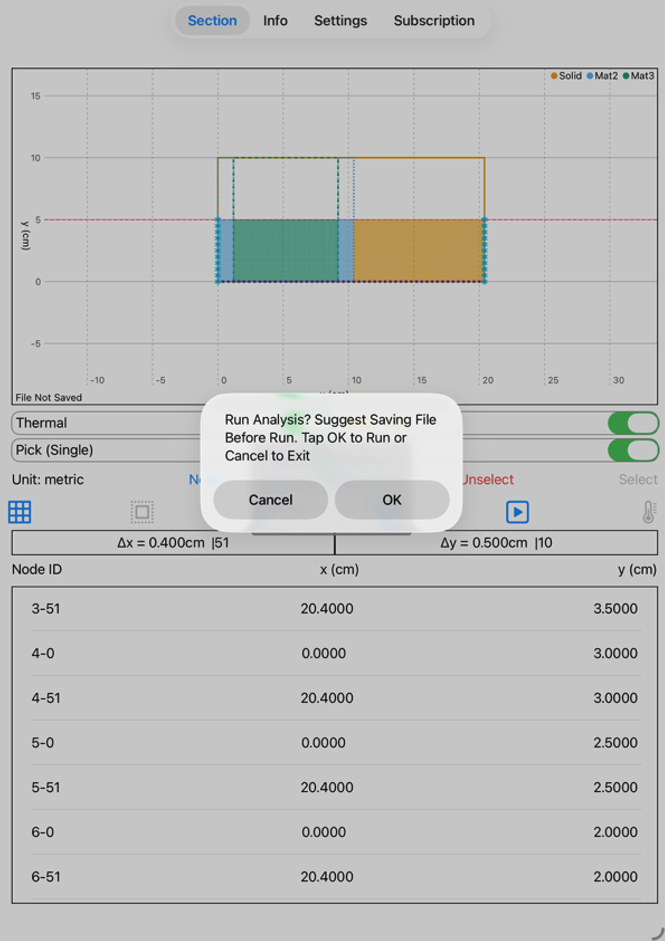
Thermal Page (Thermal Toggle button On)
Tap OK to run analysis when dialog box appears
The Results Page will automatically appear after the analysis has been completed.
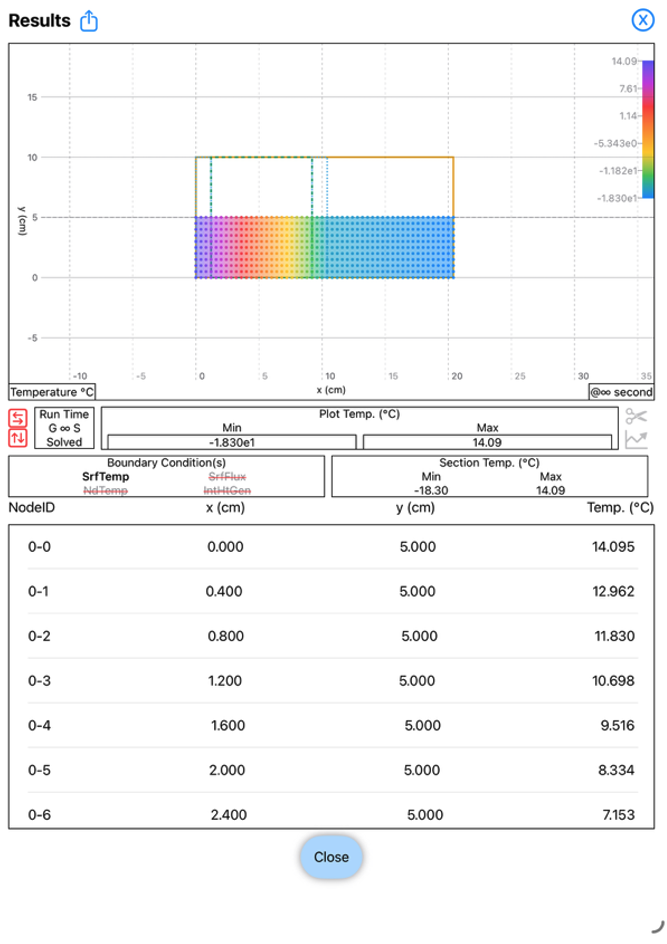
Results Page
View results
Tap the Horizontal Flux button to view the horizontal flux.
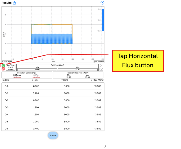
Results Page
Tap Horizontal Flux button